Machine Learning Class Notes

Subsection 2.1 Introduction

Many real world data sets lie close to a much lower dimensional manifold. Features in data sets maybe be highly correlated so there is redundant information. Features for data sets may be constructed by different groups of people and there may be some overlap. For an extreme example, suppose a measurement is recorded in both inches and centimenters as a different feature.

Reasons to reduce dimensionality.

1. Visualization. If we reduce the data to 2 or 3 dimensions then we can visualize the relationships between features.
2. Data compression will use less storage space and will speed up most learning algorithms.
3. May help to eliminate overfitting. In higher dimensional spaces, points are likely to be far apart. There may not be enough nearby points to get good results.

Problems with dimensionality reduction.

1. The performance of the learning algorithm is likely to decrease.
2. Dimensionality reduction does not remove features, it just combines all existing features into a new set of smaller features (the axes in the smaller dimensional space.) These new features will be difficult to interpret since they are a complicated combination of other features.

Example 1

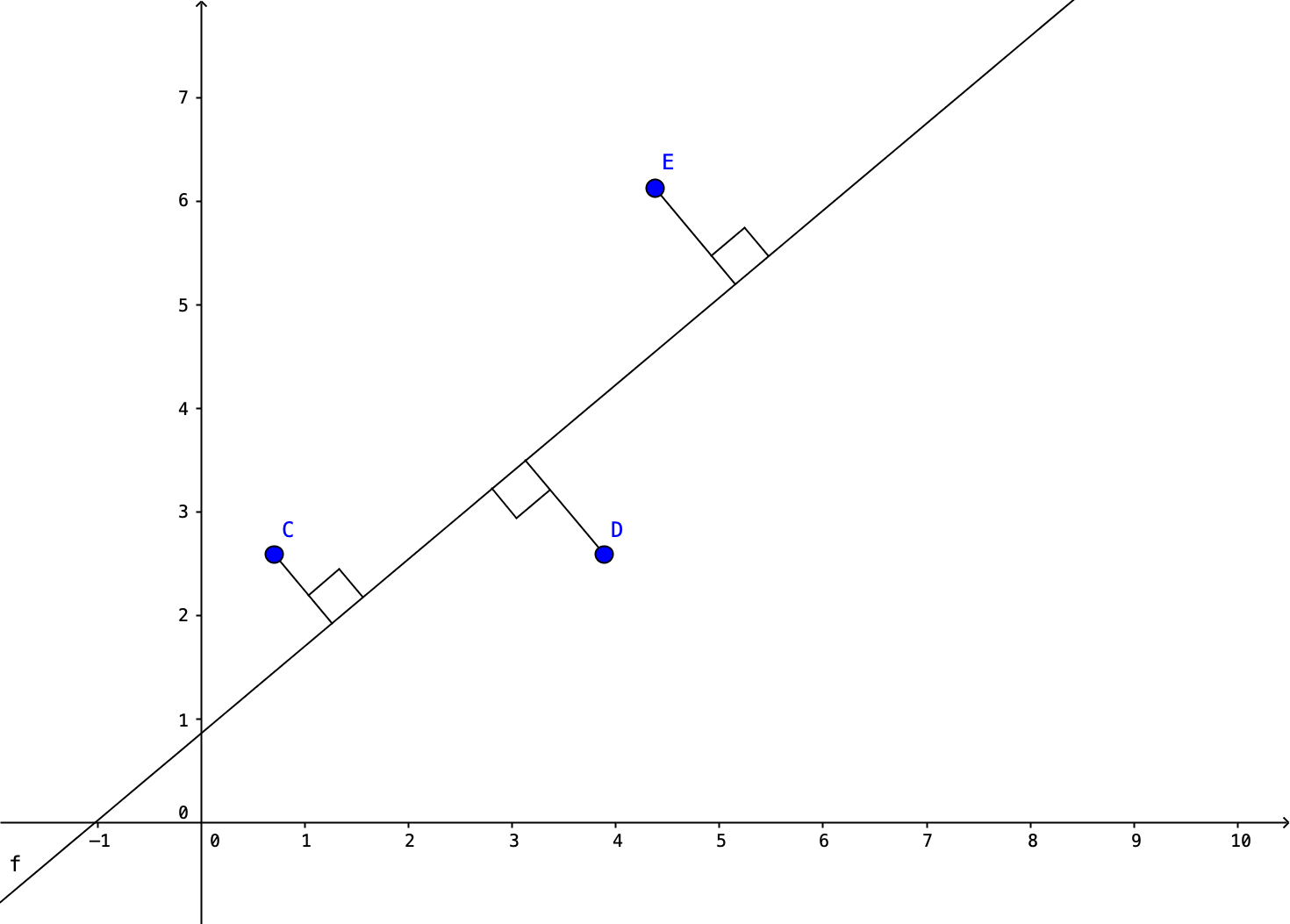
For example, suppose we have a data set with two features, a measurement in inches and a measurement in centimeters. There is some measurement error (rounding would be one way measurement error occurs) so they do not lie on a perfect line, but it is close.

We first find the line that is closest to the points. In this case we are finding the line that minimizes the orthogonal distance between the points and the line. Note other techniques, such as linear regression, minimize the vertical distance between the point and the line.

We can now project these points onto this line and reduce the 2D coordinates of the data points into a single coordinate.

This reduces the size of the data, but the new feature value does not generally correspond to anything. In this case, the new feature is very similar to the centimeter value, but it is definitely different.

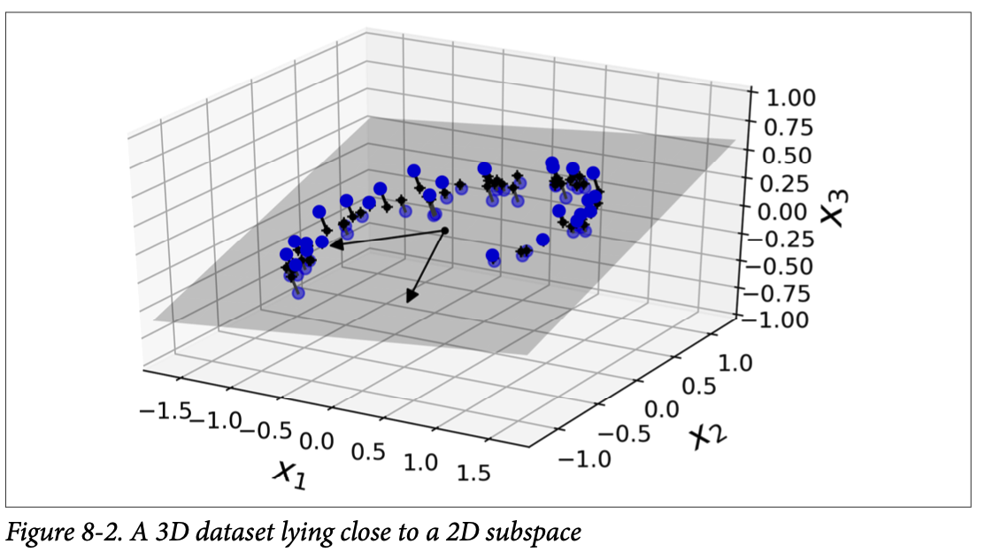
Example 2

Here's a 3D example taken from your Hands-on Machine Learning textbook. In this case, each point begins with three features \(x_1, x_2, x_3 \text{.}\) After the projection, each point has two features \(z_1, z_2 \text{.}\) These new features will most likely not have any clear connection to the original features and may not have a reasonable 'real world' interpretation.

Hands-on Machine Learning with Scikit-learn, Keras, & Tensorflow, Chapter 8

Subsection 2.2 Visualization

Let's return to the Iris data set. It has four features for each data point: petal length, petal width, sepal length and sepal width. In order to apply kNN and visualize the results, we restricted to just two of those features. What if we instead reduce the dimensionality of the data set to two dimensions? Here's a look at what happens. We'll come back and talk about all the details of the code after we discuss the ideas of the principal component analysis method of dimensionality reduction.

This looks reasonably well separated by class! You will compare how well kNN works in the homework.

Subsection 2.3 Principal Component Analysis Description

Principal Component Analysis, or PCA, is the most commonly used algorithm to implement dimensionality reduction. The idea of PCA is that we want to project the data onto a lower dimensional surface. And we want to find the lower dimensional surface that is closest to the data in terms of the mean squared distance. For example, with 2D data, we want to find the line that is closest to the data points in terms of the mean squared distance or the orthogonal distance between the points and the line. Note, that other algorithms for finding a best fit line do not necessarily use this orthogonal distance. For example, linear regression uses the vertical distance between the points to determine the best fit. This is because the goal is different in linear regression. We want to be able to predict \(y\) values in that case, so we are focusing on a single feature and maximizing our ability to predict that feature. For PCA, all features are treated equally since we are not trying to predict one of them, so we want the line that is overall closed to the data.

Steps for PCA:

1. Perform mean normalization and feature scaling so that the features have zero mean and comparable ranges of values. (Why?)
2. Identify the lower dimensional surface, or hyperplane, that is closest to the data by minimizing the mean squared area. (How?)
3. Project the data onto the lower dimensional surface. (How?)

In general, the hard part of this algorithm is Step 2. How do we determine the closest lower dimensional surface? There are two ways to think about what's happening. We want to find the closest lower dimensional surface by minimizing the mean squared distance or we want to preserve/maximize the variance after projecting onto the line.

Hands-on Machine Learning with Scikit-learn, Keras, & Tensorflow, Chapter 8

Full details for steps of PCA for a training set \(X\) with \(m \) data points and \(n \) features for each data point. That is, \(X= \{ x^{(1)},x^{(2)},\cdots ,x^{(m)} \}\) and each \(x^{(i)}\) has \(n \) features.

1. Perform mean normalization and feature scaling so that the features have zero mean and comparable ranges of values.

   1. Compute the mean

      \begin{equation*} u_j = \frac{1}{m} \sum_{i=1} ^{m} x_j ^{(i)} \end{equation*}

      and replace each

      \begin{equation*} x_j ^{(i)} \text{ with } x_j ^{(i)} - u_j \text{.} \end{equation*}

   2. If features are on different scales, then also perform feature scaling. Replace each

      \begin{equation*} x_j ^{(i)} \text{ with } \frac{x_j ^{(i)} - u_j}{s_j} \end{equation*}

      where \(s_j\) is the standard deviation, (or max-min or whatever you are using for your scaling technique.)

2. Identify the lower dimensional surface, or hyperplane, that is closest to the data by minimizing the mean squared area.

   1. Compute the covariance matrix
      \begin{equation*} \Sigma = \frac{1}{m} \sum_{i=1} ^{n} (x^{(i)}) (x^{(i)})^T \end{equation*}
   2. Compute the eigenvectors of the covariance matrix \(\Sigma \text{.}\)

   In practice, these eigenvectors can be computed most efficiently using a matrix factorization technique called Singular Value Decomposition, or SVD. SVD decomposes a training set \(X\) into three matrices

   \begin{equation*} U, s, V^T \end{equation*}

   where \(V \) is an \(n \times n \) matrix and each column is a unit vector that identifies a component of the lower dimensional space. To reduce the data to \(k \) dimensions, we pick the first \(k \) columns, also called components.

   It is possible to directly compute the covariance matrix and its eigenvalues. This will produce the same result as SVD since the covariance matrix is symmetric positive definite. However, SVD is a bit more numerically stable.

   How SVD works and why it constructs the closest lower dimensional surface to the data is beyond the scope of this class. However, it is easy enough to implement using either the numpy package or sklearn.

3. Reduce an \(n \) dimensional data set (\(n \) features, not data points) to \(k \) dimensions by projecting the data onto the lower dimensional surface. This requires only matrix multiplication. Let \(W_k\) be the first \(k \) columns of \(V\text{.}\) Then projecting the training set down to \(k\) dimensions requires computing

   \begin{equation*} X_{proj} = X W_d \text{.} \end{equation*}

   Note that \(X\) is an \(m \times n\) matrix, \(W_d\) is an \(n \times k\) matrix, so that \(X_{proj}\) is an \(m \times k\) matrix.

Subsection 2.4 PCA Implementation

We will begin with the numpy implementation of SVD for a 2D data set X. Note that c1 is the first column of Vt and the vector for the first dimension. Similarly c2 is the second column of Vt and the vector for the second dimension. To reduce this data set to 1D, we only use c1.

Code to perform SVD.

X_centered = X - X.mean(axis=0)
U, s, Vt = np.linalg.svd(X_centered)
V=Vt.T
c1 = V[:, 0] 
c2 = V[:, 1] 
print(c1)

Code to project onto one dimension.

W1 = V[:, :1]
X1D = X_centered.dot(W1)
## Or, equivalently, X1d = np.matmul(X_centered,W1)

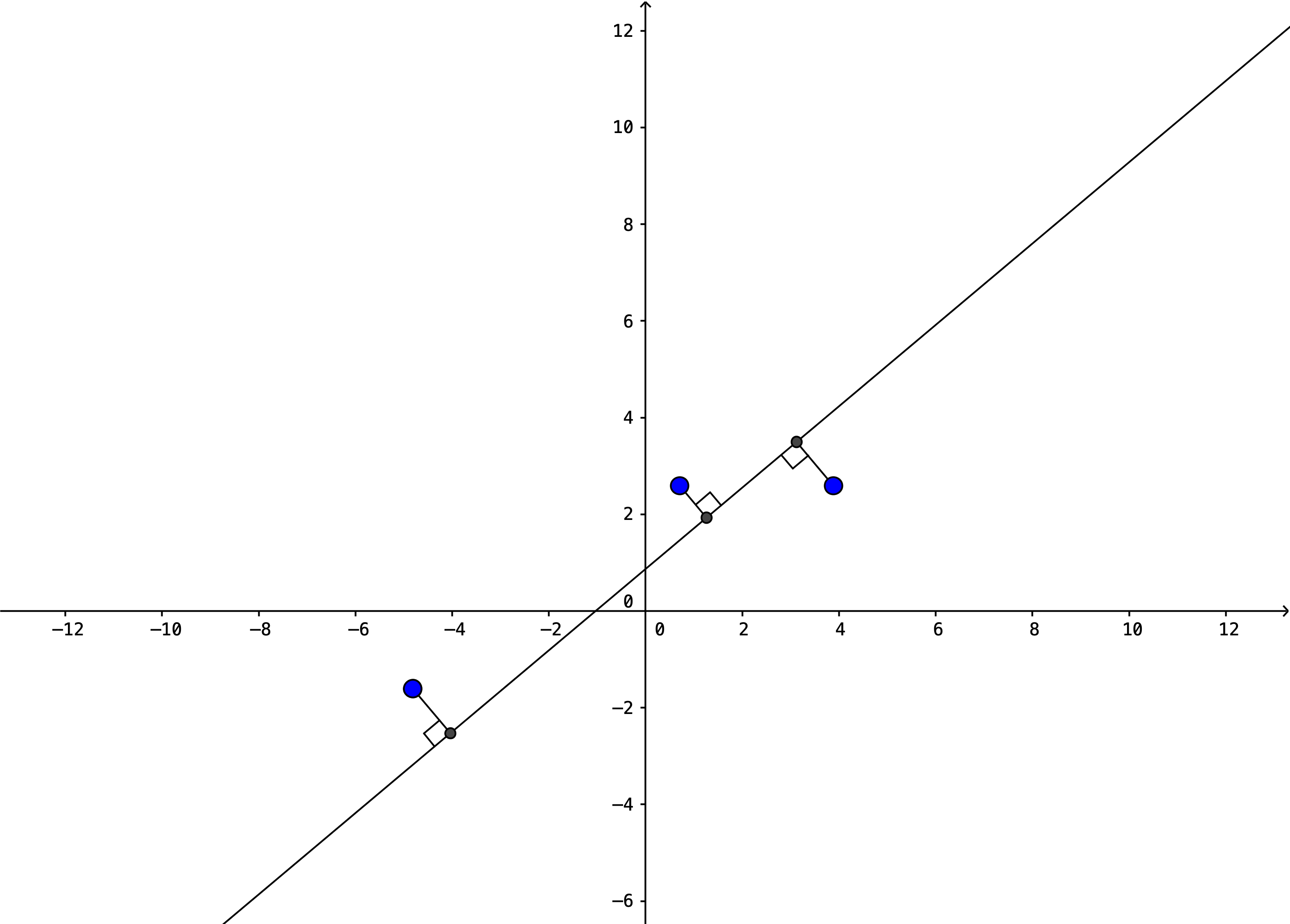
We return to our first data example and use SVD to compute the line closest to the 2D data set. We will apply mean normalization this time, but not feature scaling.

Then we project this data set onto the 1D line and plot points and line.

Implementing PCA using sklearn is even easier. It automatically performs the mean normalization.

 from sklearn.decomposition import PCA
 pca=PCA(n_components = 2)
 X2D = pca.fit_transform(X)
 

We applied this technique on the example in the Visualization Subsection.

The attribute components_ will provide the transpose of \(W_d \text{.}\) The attribute explained_variance_ratio_ will indicated the proportion of the dataset's variance that lies along each principal component. If we want to reverse the projection we can apply pca.inverse_transform(X2D).

If we are applying dimensionality reduction for visualization then we know we will need to reduce the number of dimensions to 2 or 3. However, if we are applying dimensionality reduction for data compression or speeding up other algorithms, we need to make choices about what dimension to reduce to. One option is to choose the number of dimensions that add up to a sufficiently large portion of the variance (e.g., 95%).

The following code performs PCA and computes the minimum number of dimensions required to preserve 95% of the training set’s variance:

pca = PCA(n_components=0.95) 
X_reduced = pca.fit_transform(X_train)

Another option is to plot the explained variance as a function of the number of dimensions There will usually be an elbow in the curve, where the explained variance stops growing fast. In Figure 2.6, we apply this to the MNIST digit data. You can see that reducing the dimensionality from 400 down to about 75 dimensions seems reasonable.

Hands-on Machine Learning with Scikit-learn, Keras, & Tensorflow, Chapter 8

The code for constructing the elbow is given in the github files for your text, Hands-on Machine Learning with Scikit-learn, Keras, & Tensorflow, but it runs too slowly to include here.

Subsection 2.5 PCA Variations and Caveats

There are a number of different parameters and options for PCA that are useful in practice but that we will not cover in detail. See your Hands-on Machine Learning textbook for details.

Randomized PCA will speed up SVD by approximating the first \(k\) principal components. This may be advantageous for large data sets and sklearn's default parameters will use this in certain cases.

Incremental PCA is an option if the entire dataset will not fit in memory. You can split the data into mini-batches and use an incremental PCA option.

Kernel PCA first embeds the data in a higher dimension and then applies PCA. This makes it possible to perform complex non-linear transformations. A number of different kernel options are available.

We end with a caveat. Projection is not always the best way to approach dimensionality reduction. For example, the 3D swiss roll dataset in Figure 2.7 would not respond well to a standard projection into two dimensions. While there is a 2D subspace that makes sense, this would correspond to 'unrolling' the dataset and can't be accomplished with a standard projection. Sometimes kernel PCA can help in these situations, but there are other types of dimensionality reduction, called manifold learning, that may work better in some cases. However, many of these do not scale well to large data sets.

Hands-on Machine Learning with Scikit-learn, Keras, & Tensorflow, Chapter 8