
Section 6 Parameter Tuning
All of our regression models for both classification and regression techniques, require finding values of \(\Theta\) that work well for our model and for our desired use of the data. But there are also many other parameters that we can vary as part of our optimization technique. How do we find the right mix of parameters? How do we deal with models that are overfitting and underfitting? What does it mean for a model to work well? What does desired use of the data mean? We will address various aspects of these question in this section. Regularization is an important strategy in parameter tuning to help control overfitting. Cross-validation and parameter searches are a way to help find the right mix of parameters. There are additional model evaluation metrics that are important for classification models that will help us determine if the model is working well in different situations.
Subsection 6.1 Regularization
There are three different types of error that can occur in a machine learning model: Bias, Variance, and Irreducible Error.
Irreducible Error: This is error that is inherent in the data itself. We may be able to clean up the data in the preprocessing stage, but usually there is always still some error that is present in the data.
Bias: The bias of an estimator is its average error for different training sets. If there is high bias then the model isn't doing a very good job of making predictions. Note: This is not related to the bias term in linear regression.
Variance: The variance of an estimator indicates how sensitive it is to varying training sets. If there is high variance then the model will do very well on the training set, but not very well on the testing set.
Question 6.1.
Does high bias correspond to underfitting or overfitting? What about high variance? Answer
Generally we are always trying to find a balance in our machine learning techniques between high bias and high variance. For example, in polynomial regression if the degree is too low we will have high bias and if the degree is too high we will have high variance.
Question 6.2.
What do we do if a model has high bias? What do we do if a model has high variance? Answer
Regularization is one tool to help with overfitting (high variance.) We are going to add a penalty to the cost function to constrain the size of the \(\Theta\) values. There are three different types of regularization based on the type of penalty we add to the cost function.
The first type is called Ridge Regression or \(l2\) penalty. For this technique we change the cost function to
where \(MSE(\Theta)\) stands for the mean squared error cost function for Linear Regression, but would be replaced by the appropriate cost function for the given algorithm. For example, log-loss, or cross-entropy loss for logistic regression. For Ridge Regression we penalize the \(l2\) norm in the cost function. In otherwords we try to minimize the cost function with respect to \(\theta\) values, but we add a term that penalizes the cost when the \(\theta\) values are large. Here the penalty is the \(l2\) norm or Euclidean distance from orgin. (You may also see this as \(l^2\) norm, but sklearn favors \(l2\text{.}\))
Question 6.3.
There is a new parameter \(\alpha\text{.}\) What does this do? Answer
Question 6.4.
Why does the sum start at 1 and not 0? Answer
Question 6.5.
What is the impact of adding this penalty to the cost function? What effect will it have on the \(\theta_i\) values for \(i \geq 1\text{?}\) Answer
Question 6.6.
When should we use ridge regularization? Answer
Graphs of different values of the regularization coefficient \(\alpha\) is given in Figure 6.7. 
Question 6.8.
What is regularization doing to the graph and why? Answer
There are different ways to access this in sklearn models using either ridge or l2 penalty terminology. But there are other ways to penalize the \(\theta\) values.
The second type of regularization is called Lasso Regression or \(l1\) penalty. For this technique we change the cost function to
In Lasso Regression we penalize the \(l1\) norm in the cost function. Note that again the parameter \(\alpha\) changes the amount of reglarization to do.
Question 6.9.
Why is this named Lasso? Answer
Lasso Regression tends to eliminate weights of the least important features. It is especially useful if have more features than data points. However, it can cause trouble with optimization because the gradient descent may bounce around. That is, there may be convergence issues.
Graphs of different values of the regularization coefficient \(\alpha\) is given in Figure 6.10. 
Question 6.11.
How does Lasso Regression compare to Ridge Regression (as in Figure 6.7)? Answer
Lasso Regression will be referenced in sklearn models using either lasso and l1 penalty terminology.
The third type of regularization is called ElasticNet Regression or \(l1\)-ratio. For this technique we change the cost function to
Elastic Net Regression is a mixture of Ridge and Lasso. We now have two parameters, \(\alpha\) which is the amount of regularization and \(r\) which is the mix ratio (also called the l1-ratio). The mix ratio impacts how much of ridge vs lasso you want to do. In general, \(0\lt r\lt 1\text{.}\) If \(r=1\text{,}\) then it is just Lasso. If \(r=0\text{,}\) then it is just ridge
In general, Ridge Regression is a good default (\(r=0\)). Lasso Regression is good if you suspect that you only have a few good features (\(r=1\)). Elastic Net is prefered over Lasso when several features are strongly correlated or the number of features is greater than the number of training instances.
Early stopping is another way we can try to reduce overfitting. We train the data until the testing score starts getting worse. The steps for this method are
- Train data in epochs.
- Track training and testing errors.
- Stop once you start doing worse on testing.
For example, in Figure 6.12 we would stop training after approximately 240 epochs. 
This is usually one of the parameters you can choose in many of the machine learning models. That is, you can often apply this by choosing early_stopping=True.
See Jupyter notebook for details on implementation for these techniques.
Subsection 6.2 Parameter Searching
We now have many parameters for our models that we want to explore and we would like a way to find the best parameter or combination of parameters. Generally this requires separating testing data and measuring the performance of our model on the testing data and comparing its performance across parameters. We are going to talk about ways to do that more efficiently.
The first issue we have seen with this technique is that the way the data is split between training and testing can really impact performance and accuracy of a model. However, sometimes we have small data sets, so it can be hard to do this well. One technique we can apply to help with this is called \(k\)-fold cross validation. In this technique we break the data into \(k\) sets, use each set as test data, and the remaining data as training data. We create the model \(k\) different times, (on \(k\) different training set), examine all the scores and the average score.
Example 6.13.
Suppose the data set has 500 elements and we want to apply 5-fold cross validation. We separate the data into five folds where each fold has a random selection of 100 data points.
| 100 | fold 1 |
| 100 | fold 2 |
| 100 | fold 3 |
| 100 | fold 4 |
| 100 | fold 5 |
Question 6.14.
If our 500 data points have 300 dogs and 200 cats, how should we distribute them across folds? AnswerOf course, sklearn has a built-in for this its cross_val_score.
from sklearn.neighbors import KNeighborsClassifier
from sklearn.model_selection import cross_val_score
knn = KNeighborsClassifier(n_neighbors = 3)
cv_scores = cross_val_score(knn, X, y, cv=3)
The full list of parameters are here:
cross_val_score(estimator, X, y=None, groups=None, scoring=None,
cv=None, n_jobs=None, verbose=0, fit_params=None,
pre_dispatch='2*n_jobs', error_score=nan)
The main ones we will use are
- The
estimatoris the machine learning technique (kNN, PCA, LinearRegression (with or without polynomial features), LogisticRegression (with or without polynomial features), etc) that we want to apply to the data. - \(X\) is the set of features for our data (should be scaled!).
- \(y\) is the labeled data if a supervised tecnique is being used. No \(y\) is entered if using an unsupervised technique.
-
scoring=Nonemeans the estimators default scoring method is used. -
cvis the number of folds. (The default,cv=Noneusing 5 folds.) If the estimator is a classification technique then the data is split into folds using a stratified method. A random split is used for regression techniques.
Question 6.15.
What percentage of the data is in a testing set if five folds are used? Answer
Question 6.16.
What does stratified mean? Answer
Question 6.17.
What are the pros and cons of cross validation? Answer
Remember that when feature scaling is applied to data, it should only be done on the training data and not the full data set. Otherwise it leaks data about the testing set. For cross validation it must be done on each training set individually. (The PIPELINE feature will really help here!)
We will return to the fruit data set from exam 1 for an example of cross validation.
We are going to revisit kNN as our classification technique and use all four features. Since the scales of the features are quite different, it is very important to use feature scaling now. We will create a Pipeline to combine ScandardScaler and kNeighborsClassifier.
Question 6.18.
What happens if we use six folds? Answer
Question 6.19.
How many folds should we use in cross validation? Answer
Nearly all of the models have multiple parameters to tune. How do we find the best combination of parameters? For example, in the previous fruit data set example, what is the best value of \(k\) to use in \(k\) nearest neighbors? For a single parameter, we can use a validation curve. A validation_curve will produce an \(m \times n \) array of scores for training and testing where \(m= \) the number of parameters specified in the range and \(n= \) the number of folds for cross validation. We can then graph an average score across folds to see how the score varies as we change the single parameter.
from sklearn.model_selection import validation_curve
param_range = range(1,8,2)
train_scores, test_scores = validation_curve(KNeighborsClassifier(), X, y,
            param_name='n_neighbors', param_range=param_range, cv=cvnum)
The full list of parameters is
validation_curve(estimator, X, y, param_name, param_range,
	groups=None, cv=None, scoring=None, n_jobs=None,
	pre_dispatch='all',verbose=0, error_score=nan).
Most of these are the same as cross_val_score():
- The
estimatoris the machine learning technique (kNN, PCA, LinearRegression (with or without polynomial features), LogisticRegression (with or without polynomial features), etc) that we want to apply to the data. - \(X\) is the set of features for our data
- \(y\) is the labeled data if a supervised tecnique is being used. No \(y\) is entered if using an unsupervised technique.
-
scoring=Nonemeans the estimators default scoring method is used. -
cvis the number of folds. (The default,cv=Noneusing 5 folds.) If the estimator is a classification technique then the data is split into folds using a stratified method. A random split is used for regression techniques.
The new ones are param_name and param_range where we specify the parameter we want to vary.
Example 6.20.
If we call
train_scores, test_scores = validation_curve(KNeighborsClassifier(), X, y,
param_name='n_neighbors',param_range=[1,3,5,7], cv=3).
This will produce an \(m \times n \) array of scores for training and testing where \(m \) is the number of parameters specified in the range and \(n \) is the number of folds for cross validation.
| fold 1 | fold 2 | fold 3 | |
| k=1 | |||
| k=3 | |||
| k=5 | |||
| k=7 |
Let's try it!
Now that we have all the scores, it is easiest to analyze them with a plot. We will plot the average across folds as the number of neighbors increases.
Question 6.21.
What do we think of our model? What's the best value of \(k\text{?}\) Is this model a keeper? Answer
Question 6.22.
Why is this model not very good? Answer
Note that we have to call the parameter name differently now. Its the name we used in the Pipeline for KNeighborsClassifer() and double underscore to reference the parameter.
We can search over multiple parameters with a parameter search. The main techniques combine cross validation with either an exhaustive search over all combinations of parameters in GridSearchCV or random search over combinations of parameters in
RandomizedSearchCV. We will begin with GridSearchCV. This will perform an exhaustive search over all combinations of parameters entered, each combination calculated over \(cv\) folds. The full parameter list is
 from sklearn.model_selection import GridSearchCV
 GridSearchCV(estimator, param_grid, scoring=None, n_jobs=None,
    iid='deprecated', refit=True, cv=None, verbose=0,
    pre_dispatch='2*n_jobs', error_score=nan, return_train_score=False)
Most of these should look familiar. We specify the parameters we want to examine with a dictionary for param_grid. We can access the parameters that return the best score on the testing set with grid_knn_acc.best_params_ and their corresponding scores in grid_knn_acc.best_score_. Note that the default setting will not return the scores on the training data to reduce the number of calculations made. It is still useful to compare training and testing scores, but it may be better to go back and do that on just the best model rather than storing all the scores on the training data. A full set of results cana be obtained with grid_knn_acc.cv_results_.
Example without a Pipeline and with only one parameter.
Question 6.23.
What's up with the rankings? Is \(k=3\) really the best? Answer
Example with a Pipeline and two parameters.
Question 6.24.
How many times did knn_model create a different model in the above GridSearchCV? Answer
Depending on the size of our model, an exhaustive grid search, might not be the way to go. Another option is
RandomizedSearchCV. A fixed number of parameter values are examined here (specified by n_iter=10.) Parameters are specified with a dictionary or list of dictionaries in param_distributions. Ranges may be specified as a list (recommended for discrete parameters) or a distribution (recommended for continuous parameters). We'll mostly stick to lists of ranges for parameters. The full list of parameters is
 RandomizedSearchCV(estimator, param_distributions, n_iter=10,
    scoring=None, n_jobs=None, iid='deprecated', refit=True,
    cv=None,verbose=0, pre_dispatch='2*n_jobs', random_state=None,
    error_score=nan, return_train_score=False)
Let's examine a different classification technique. Let's apply LogisticRegression to the fruit data set and examine the effects of regularization. Note that the regularization parameter for Logistic Regression is C where \(C=\frac{1]{\alpha}\text{.}\) So large values of C indicate small amounts of regularization. We usually want to vary C by powers of ten. How do you think Logistic Regression will do compared to k Nearest Neighbors?
Question 6.25.
What does the notation 1e-30 mean? Which method does better? Why? Answer1e-30 indicates scientific notation so \(1 \times 10^{-30}\text{.}\) k Nearest Neighbors did better. Possibly linear decision boundaries don't make sense on this data set. Maybe we should try LogisticRegression with Polynomial features?
Subsection 6.3 Evaluating Classification Models
As we are adding models to our collection, how do we determine which is the best one for our data? What does best even mean? For classification models, examining the accuracy of the model is always a good score to examine, but it may not help us determine the best model for our situation.
Question 6.26.
Suppose we have a fruit data set with 45 apples and 5 oranges. If our model is 90% accurate, is that a good score? Answer
Some other model evaluation techniques that are often used include Confusion Matrices, Precision vs Recall graphs, and ROC curves.
A Confusion Matrix records how accurate our model is in each class relative to each other class. For two classes, there are four categories,
- True Negative (TN): The data has class 0 and the algorithm predicts class 0.
- False Negative (FN): The data has class 1 and the algorithm predicts class 0.
- False Positive (FP): The data has class 0 and the algorithm predicts class 1.
- True Positive (TP): The data has class 1 and the algorithm predicts class 1.
and we can visualize this as a \(2 \times 2\) matrix.
| predict 0 | predict 1 | |
| class 0 | TN | FP |
| class 1 | FN | TP |
For \(k\) classes, we can visualize this as a \(k \times k\) matrix. Note TN,FP,FN,TP no longer make sense in this case as there are many more than four cases.
| predict 0 | predict 1 | \(\cdots \) | predict k | |
| class 0 | ||||
| class 1 | ||||
| \(\vdots \) | ||||
| class k |
In the last example for logistic regression, even our best model didn't do very well. Why not? For simplicity we are looking at the confusion matrix on the full data set, but really we should only be looking at it on the testing data.
Question 6.27.
What fruits is this model having difficulty predicting? How does this help us build a better model? Answer
Question 6.28.
What is the accuracy of the model? How many did the model get wrong? What fraction of the oranges were correctly predicted to be orange? What fraction of the fruits predicted to be oranges are really oranges? Answer
The trade-off between Precision and Recall is usually a function of our parameter tuning. We often want to analyze this to choose the best model based on how we are going to be using the data.
The term Recall (also called True Positive Rate) is defined as \(\frac{\text{TP}}{TP+FN}\) for two classes. In general, this involves all entries in the row for class 1 (orange). What fraction of positive instances are correctly predicted as positive?
The term Precision (also known as Positive Predictive Value) is defined to be \(\frac{\text{TP}}{TP+FP}\) for two classes. In general, this involves all entries in the column for predicting class 1. What fraction of positive predictions are correct?
In some cases precision might be more important than recall and vice versa.
Question 6.29.
Suppose we are using machine learning to diagnose tumors and class 1 indicates a malignant tumor and class 0 indicates a tumor is not malignant (benign). What does recall mean in this case? What does precision mean in this case? Are they equally important or is one of them more important? Answer
Question 6.30.
Suppose we are using machine learning to predict if an email is spam (class 1) or not (class 0). What does recall mean in this case? What does precision mean in this case? Are they equally important or is one of them more important? Answer
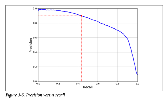
Ideally, we would like both precision and recall to be 100%, but generally as we vary the parameters, some parameters will have better precision at the expense of recall and vice-versa. Thus, we can examine precision versus recall scores to determine the parameters that give us the best model based on the desired use of the model/data.
We can also graph precision versus recall as parameters are varying. But this only works with binary classes.from sklearn.metrics import precision_recall_curve
A sample precision versus recall curve from your textbook is below.
The term True Positive Rate = TPR (same as Recall) is defined as \(\frac{\text{TP}}{TP+FN}\) for two classes. In general, this involves all entries in the row for class 1. What fraction of class 1 is correctly predicted to be class 1?
The term False Positive Rate =FPR (also known as the probability of false alarm) = \(\frac{\text{FP}}{FP+TN}\) In general, this involves all entries in the row for class 0. What fraction of class 0 is incorrectly predicted to be class 1?
A ROC Curve (stands for Receiver Operator Characteristic Curve) is created by plotting the True Positive Rate as a function of False Positive Rate as various parameters are varied. (FPR on \(x\)-axis, and TPR on \(y\)-axis.) It was originally developed for operators of military radar receivers. In this case we are trying to find a balance between correctly detecting an event and detecting false alarms. Ideally, we want the TPR to be 100% and FPR to be 0%. However, normally as we vary parameters we can only detect all the true positives if we allow some false alarms, and we can only have no false alarms with a very poor ability to detect the desired event. Thus, we want to identify a model that corresponds to an appropriate trade-off between detection and false alarms that is determined by the given situation. 
ROC curves are generally better when observations are balanced across classes. Precision-Recall Curves are generally better for imbalanced data sets.