
Section 4 Logistic Regression
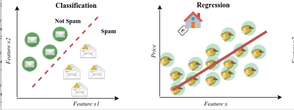
The goal for logistic regression is to modify linear regression to use it for classification instead of regression. (Yes, but its still called regression!) Remember for classification we want to predict classes instead of a range of values. Some examples of classification include:
- Predicting if an email is spam or not spam.
- Predicting if an online transaction is fraudulent or not.
- Predicting if a patient has a malignant or benign tumor.
- Predicting the type of iris or fruit.
Subsection 4.1 Steps of Linear Regression
We begin with a review of the steps of Linear Regression so that we can discuss the modifications needed for Logistic Regression.
-
Data.
Identify features and labels in the data. Features are encapsulated in the \(m \times (f+1)\) matrix, \(X\text{,}\) and labels in the \(m \times 1\) matrix, \(y\) where the values in \(y\) occur in a continuous range.
\begin{equation*} X= \left[ \begin{matrix} 1 \amp x_1^{(1)} \amp x_2^{(1)} \amp x_3^{(1)}\amp \cdots \amp x_f^{(1)}\\ 1 \amp x_1^{(2)} \amp x_2^{(2)} \amp x_3^{(2)}\amp \cdots \amp x_f^{(2)}\\ \amp \amp \amp \vdots \amp \amp \\ 1 \amp x_1^{(m)} \amp x_2^{(m)} \amp x_3^{(m)}\amp \cdots \amp x_f^{(m)}\\ \end{matrix} \right] \text{ and } y= \left[ \begin{matrix} y^{(1)}\\ y^{(2)}\\ \vdots \\ y^{(m)}\\ \end{matrix} \right] \end{equation*} -
Learn Function.
Learn a function \(F\) such that \(F(X) \approx y \text{.}\)
-
Choose a Model.
For linear regression we assume a linear model for \(F(X)\text{.}\)
\begin{equation*} F(X)=h_\Theta(X)={X}{\Theta} = \left[ \begin{matrix} 1 \amp x_1^{(1)} \amp x_2^{(1)} \amp x_3^{(1)}\amp \cdots \amp x_f^{(1)}\\ 1 \amp x_1^{(2)} \amp x_2^{(2)} \amp x_3^{(2)}\amp \cdots \amp x_f^{(2)}\\ \amp \amp \amp \vdots \amp \amp \\ 1 \amp x_1^{(m)} \amp x_2^{(m)} \amp x_3^{(m)}\amp \cdots \amp x_f^{(m)}\\ \end{matrix} \right] \left[ \begin{matrix} \theta_0\\ \theta_1\\ \vdots \\ \theta_f\\ \end{matrix} \right] \end{equation*} -
Cost Function.
We define what \(F(X) \approx y \) means with a cost function. We used the mean squared error cost function.
\begin{equation*} J = \frac{1}{2m} \sum_{i=1}^m \left[ h_\theta(x_1^{(i)},x_2^{(i)}, \cdots, x_f^{(i)}) - y^{(i)} \right]^2 = \frac{1}{2m}(X\Theta-y)^T(X\Theta-y)\text{.} \end{equation*}The goal is to find \(\Theta \) by minimizing \(J \text{.}\)
-
Solve for \(\Theta\)
How do we actually find \(\Theta \text{?}\)
Option 1: Solve for \(\Theta \) exactly by setting the partial derivatives of the cost function equal to 0. This leads to the normal equation. This is (almost) the strategy for sklearn's LinearRegression. (It calculates pseudoinverses rather than exact inverses for computational efficiency.)
Option 2: Approximate \(\Theta \) with an optimization technique such as gradient descent. This is (almost) the strategy for sklearn's SGDRegressor. (Its really stochastic gradient descent, only calculating the derivative at random points rather than using the entire feature matrix.)
Question 4.1.
When should we use LinearRegression versus SGDRegressor? AnswerThis is primarily based on the size of the data. LinearRegression works well for smaller data sets (maybe hundreds of data points), but larger data sets will need SGDRegressor. -
Make Predictions!
Use \(\Theta \) to predict values for new data points by plugging \(X_{new}\) into \(F(X)\text{.}\)
\begin{equation*} y_{new}=F(X_{new})=h_\theta(X_{new})={X_{new}}{\Theta} \end{equation*}
Question 4.2.
Which of these six steps do you think need to be changed to apply classification instead of regression?
AnswerData. The values in \(y\) must occur in a discrete range instead of a continuous range.
Learn Function. Still want to learn a function!
Linear Model. Hmmm. Is a linear model still a good model to predict a class? We should think about that.
Cost Function. Hmmm. Is mean squared error still a good cost function? We should think about that.
Solve for \(/Theta\text{.}\) Can we solve for \(/Theta\) by setting partial derivatives of the cost function equal to 0? Should we use optimization techniques like gradient descent? Will gradient descent still work here? We will have to come back to this question after we make some decisions about our cost function.
Make Predictions! The predictions need to be a class not a value. We will need some way to interpret the output of our function \(F(X) \) as a class.

So clearly there's a lot to think about to use this same model for classification (logistic regression) instead of linear regression. Let's examine each of the six steps carefully.
Subsection 4.2 Data
For linear regression: Identify features and labels in the data. Features are encapsulated in the \(m \times (f+1)\) matrix, \(X\text{,}\) and labels in the \(m \times 1\) matrix, \(y\) where the values in \(y\) occur in a continuous range.
Change needed! We need to specify \(y\) values so that they indicate a class. For example, to determine if a message is spam or not spam, \(y_i \in \{0,1\}\) where 0 usually indicates the negative class (not spam) and 1 usually indicates the positive class (spam). In the iris data set, \(y_i \in \{0,1,2\}\) for the three different types of irises. We will start by focusing on the case with two classes, but eventually we will generalize to the multiclass case.
Remember the column of ones corresponded to the bias term in our model, so we'll have to come back to the format for \(X\) after we talk about our model.
Subsection 4.3 Learn Function
For linear regression: Learn a function \(F\) such that \(F(X) \approx y \text{.}\)
No change needed! We still want to learn a function \(F\) such that \(F(X) \approx y \text{.}\)
Question 4.3.
When will this NOT be true in machine learning?
AnswerThis is always going to be the case for supervised machine learning, but will not be the case for unsupervised machine learning. (There are no labels to learn!) Although usually we are still trying to learn a function.
Subsection 4.4 Choose a Model.
For linear regression: For linear regression we assume \(F\) is linear and \(F(X)=h_\Theta(X)={X}{\Theta}\text{.}\) Does linear still make sense?
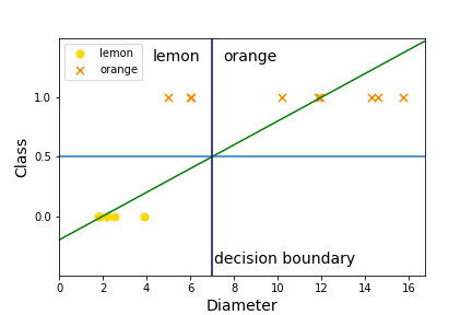
Suppose we are trying to identify the type of fruit in a data set. For simplicity, we will assume there are only two fruits, lemons and oranges, and only one feature, the diameter of the fruit. Let's start by making up some data!
Suppose we model this with a linear function. Let's use linear regression! Our data set is super small so LinearRegression will be the right choice.
Question 4.4.
Does this seem like a good way to predict if the fruit is a lemon or an orange? What problems do you see with this technique? If the diameter of a fruit is 3 what will this model predict? What if the diameter of the fruit is 8?

If we use our linear model \(y(x)=.25*x-.41\) on our test points, then \(y(3)=.25*3-.41=0.34\) and \(y(8)=.25*8-.41=1.59\text{.}\) What should we do with those values?
We need a way to convert the \(y\) value of the function to predict a class rather than a continuous range of values. We can convert this to zeros and ones, by setting a threshold, say halfway between 0 and 1. That is, we can predict a class as follows:
If we use this threshold then we would predict lemon for \(x=3\) and orange for \(x=8\text{.}\) This seems reasonable. But how well does the linear function do on the training data. Let's add the threshold to our graph and decision boundary to the graph.
Its not perfect on this data set, but it isn't so bad. However, it could be really terrible on a data set.
Question 4.5.
Easy question: Is this a linear model? Hard question: Can anyone give me a function that has this shape?
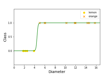
Another problem with a linear model is that it will predict values from \(-\infty\) to \(\infty\) and it would really make more sense to only produce values in the 0 to 1 range. Thus, we are not happy with a linear model anymore. We want to adapt the model so that \(0 \leq h_\Theta(X) \leq 1\text{.}\) We will keep a linear piece, but add a new function on top to keep the range between 0 and 1.
Old: \(h_\Theta(X)={X}{\Theta}\)
New: \(h_\Theta(X)=g({X}{\Theta})\)
Question 4.6.
What is the shape of \({X}{\Theta}\text{?}\)
AnswerX.shape=(m,f+1) and Theta.shape=(f+1,1). Thus, \({X}{\Theta}\) is a \(1 \times 1\) matrix! So \(g(z)\) is just a single variable function!
New function \(g\text{:}\) Use Sigmoid or Logistic function for \(g(z)\text{.}\)
Question 4.7.
Calculus Quiz: What is
Let's graph it!
Hooray! This has the shape we are looking for!
Change needed! We replace \(h_\Theta(X)\) with a combination of a logistic model and a linear model.
Question 4.8.
We've specified our model now. Do we still need the columns of ones in our data \({X}\text{?}\)
AnswerYes! The linear piece \({X}{\Theta}\) is the same as before so we still need the column of ones in \({X}\) for the bias terms, \(\theta_0\text{.}\) BUT most sklearn functions (like LinearRegression, SGDRegressor) will do this automatically for us, so we don't normally need to actually add this to the data.
Subsection 4.5 Cost Function
For linear regression: Solve for \(\Theta \) so that \(F(X)=h_\Theta(X) \approx y \text{.}\) We define what \(F(X) \approx y \) by minimizing a cost function. We used the mean squared error cost function.
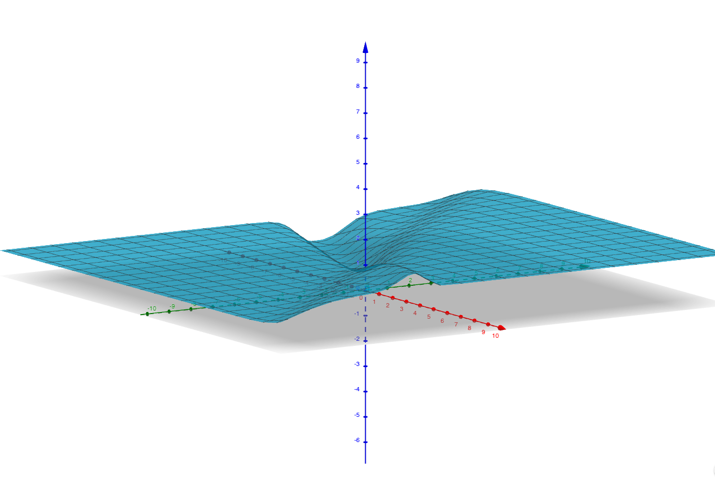
Is this still a good cost function? Remember for the purposes of gradient descent (and other optimization strategies) we want a smooth, convex (concave up) cost function so we can easily find a global minimum.
In the previous step to decide on a model we changed our model to be
For this model the mean squared error cost function is
Question 4.9.
Is this still a nice smooth, convex function? Can we minimize this function easily?
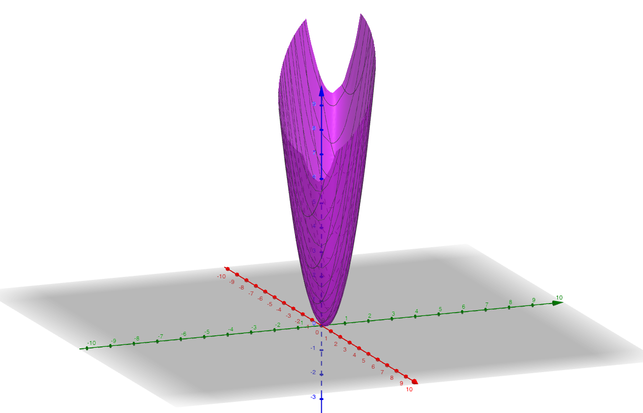
Example 4.10.
Let's look at a small example to explicitly see what this cost function looks like. Let
So we are trying to solve for
that will minimize the cost function \(J\)
Does this seem like a nice function to minimize?
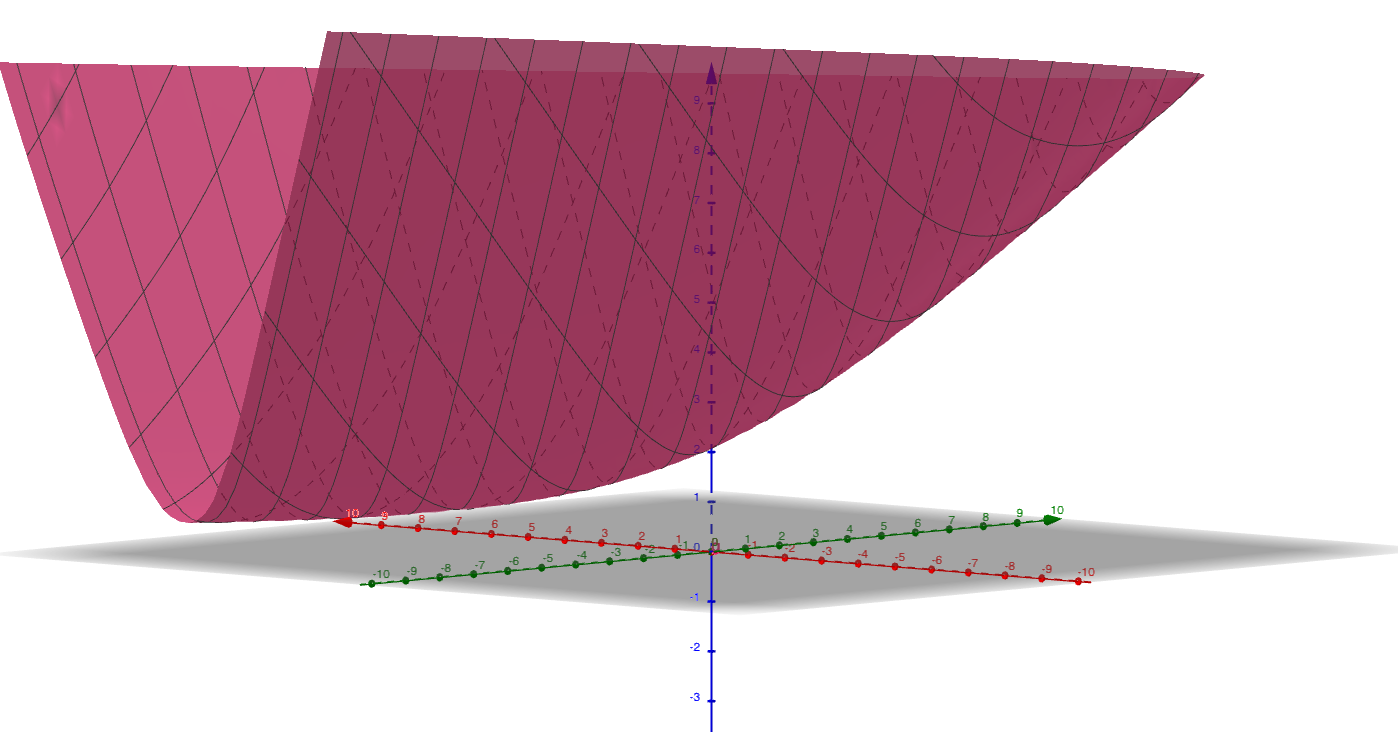
Just for comparison, in the old linear case, we would have something like
This is a nice smooth convex function!
Looks like we need a new cost function! We will turn to statistics and the principle of maximum likelihood estimation to derive a nice, convex cost function. (Ok, we'll skip the derivation but here it is!)
where
NOTE: log(\(z\)) means NATURAL LOG in this case. That is, \(\log(z)\) means log base \(e\text{,}\) not log base 10, or (\(\log(z)=\ln(z)\)).
So we won't go through the entire derivation of this function, but let's think about why these make sense. Remember that
is chosen so that \(0 \leq h_\Theta(X) \leq 1\text{.}\) Let \(w= h_\Theta(X)\) and restrict the domain to \(0 \leq w \leq 1\text{.}\) Then we are interested in
Let's graph it to see what happens in this domain \(0 \leq w \leq 1\text{.}\)
Using the graph we can see that
- GREEN POINT: if \(y=1\) and \(h_\Theta(X)=1\) (prediction is correct!) then the \(\operatorname{Cost}(X,y)=-log(1)=0\text{.}\)
- RED POINT: if \(y=1\) and \(h_\Theta(X)=0\) (prediction is completely wrong!) then the \(\operatorname{Cost}(X,y)=-log(0)= \infty\text{.}\)
- BLUE POINT: if \(y=0\) and \(h_\Theta(X)=0\) (prediction is correct!) then the \(\operatorname{Cost}(X,y)=-log(1-0)=0\text{.}\)
- HOT PINK POINT: if \(y=0\) and \(h_\Theta(X)=1\) (prediction is completely wrong!) then the \(\operatorname{Cost}(X,y)=-log(1-1)= \infty\text{.}\)
Of course, \(h_\Theta(X)\) probably won't predict exactly 0 or 1, but if it is close to the correct prediction then the cost will be small and if it is far from the correct prediction then the cost will be large.
The only problem left in this cost function is that it is a piecewise function and that is inconvenient. But since \(y=0\) and \(y=1\) are the only possible values for \(y\text{,}\) we can combine them into a single function.
Change Needed! New Cost Function
Note that if \(y_i=1\) then \((1-y_i)\log(1-h_\Theta(X{(i)})) =0\) and if \(y_i=0\) then \(y_i\log(h_\Theta(X^{(i)})) =0 \text{,}\) so that this is the same definition as our piecewise function.
But is this function smooth and convex so that we can optimize it? Let's return to Example 4.10 and compute the cost with the new cost function.
So much nicer! We are now ready to solve for \(\Theta \) by minimizing \(J \text{.}\)
Subsection 4.6 Solve for \(\Theta\)
For linear regression: Solve for \(\Theta \) by setting the partial derivatives of the cost function equal to 0 or approximate \(\Theta \) with an optimization technique such as gradient descent.
Question 4.11.
What should we do now? Answer
Subsection 4.7 Make Predictions
For linear regression: Use \(\Theta \) to predict values for new data points by plugging \(X_{new}\) into \(F(X_{new})\) so that
This won't quite work in our logistic case. Remember that \(0 \leq h_\Theta(X) \leq 1\) but it will normally return a value that is not either 0 or 1.
Change needed! Instead we interpret \(h_\Theta(X)\) as the probability that \(y=1\text{.}\) More precisely we mean \(h_\Theta(X)\) is the probability that \(y=1\) given the data \(X\) and the model \(y\text{.}\) In the notation of probability:
Note that \(P(y=0 \mid X,\Theta)\) can easily be calculated as \(1-P(y=1 \mid X,\Theta)\text{.}\) That is, the probability that \(y=0\) is the probability that \(y\) is not 1.
Question 4.12.
In our lemon and orange example, what would we predict if \(h_\Theta(X)=.7\text{?}\)
AnswerIf \(h_\Theta(X)=.7\text{,}\) there is a 70% probability that \(X\) is an orange so we would (most likely) predict orange in this case.

Hopefully, we now understand the idea of logistic regression. Let's summarise our steps and try to understand the output of our model. That is, we've done a bunch of work to find \(\Theta\text{,}\) what does it tell us?
Question 4.13.
What did \(\Theta\) tell us in linear regression?
AnswerThe coefficients of a line that modeled our training data, \(y \approx \theta_0 +\theta_1 x_1 + \cdots \theta_f x_f \text{.}\) Should we still get the coefficients of a line that models our training data in logistic regression? Should we still get the coefficients of a line?
Subsection 4.8 Steps for Logistic Regression
-
Data.
Identify features and labels in the data. Features are encapsulated in the \(m \times (f+1)\) matrix, \(X\text{,}\) and labels in the \(m \times 1\) matrix, \(y\) where the values in \(y\) occur in a discrete range, so far we have only discussed \(y_i \in \{0,1\}.\)
\begin{equation*} X= \left[ \begin{matrix} 1 \amp x_1^{(1)} \amp x_2^{(1)} \amp x_3^{(1)}\amp \cdots \amp x_f^{(1)}\\ 1 \amp x_1^{(2)} \amp x_2^{(2)} \amp x_3^{(2)}\amp \cdots \amp x_f^{(2)}\\ \amp \amp \amp \vdots \amp \amp \\ 1 \amp x_1^{(m)} \amp x_2^{(m)} \amp x_3^{(m)}\amp \cdots \amp x_f^{(m)}\\ \end{matrix} \right] \text{ and } y= \left[ \begin{matrix} y^{(1)}\\ y^{(2)}\\ \vdots \\ y^{(m)}\\ \end{matrix} \right] \end{equation*}Open Question: What if there are more classes?
-
Learn Function.
Learn a function \(F\) such that \(F(X) \approx y \text{.}\)
-
Logistic Model
For logistic regression we assume \(F\) is logistic but with an inner linear component.
\begin{equation*} F(X)=h_\Theta(X)=g({X}{\Theta})= \frac{1}{1+e^{-{X}{\Theta}}}. \end{equation*} -
New Cost Function.
Solve for \(\Theta \) so that \(F(X) \approx y \) by minimizing the cost function
\begin{equation*} J = \frac{1}{m} \sum_{i=1} ^m \operatorname{Cost}(h_\Theta(X),y) \end{equation*}\begin{equation*} = -\frac{1}{m} \sum_{i=1} ^m y_i\log(h_\Theta(X^{(i)})) +(1-y_i)\log(1-h_\Theta(X{(i)})) \text{.} \end{equation*}Remember \(y_i \in \{0,1\}\) in order for this to work. So we might have to change this if there are more class.
-
Optimization Technique.
Use some optimization technique.
Open Question: What optimization technique?
-
Make Predictions!
Use \(\Theta \) to predict values for new data points by interpreting \(h_\Theta(X)\) as the probability that \(y=1\text{.}\) That is,
\begin{equation*} h_\Theta(X)=P(y=1 \mid X,\Theta). \end{equation*}
Subsection 4.9 Understanding \(\Theta\)
We first discuss how to make a prediction for the class of \(X\text{.}\) Remember that we interpret \(h_\Theta(X)\) as the probability that \(y=1\text{.}\) To convert this into predicting a class, we generally set a threshold of 0.5. That is, we would predict
Since \(h_\Theta(X)=g(X\Theta)\) where \(g\) is the sigmoid function, this threshold corresponds to
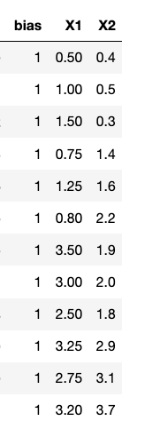
Example 4.14.
Let's look at a simple example to see all of this in action. Suppose we have a data set with two features, two classes and twelve data points.
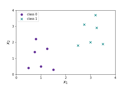
We want to find
so that
is minimized. Suppose we do and we find
I made these numbers up. We'll compare to actual logistic regression shortly.
Question 4.15.
What does this tell us? When will we predict \(y=1\text{?}\)
AnswerIn order for \(h_\Theta(X) \geq 0.5\) we need \(X\Theta \geq 0\text{.}\)
We want to know where \(-7+3x_1+x_2 \geq 0 \text{.}\) Solving for \(x_2 \) gives \(x_2 \geq 7-3x_1 \text{.}\) \(x_2 = 7-3x_1 \) is a line, so we will have a linear decision boundary! 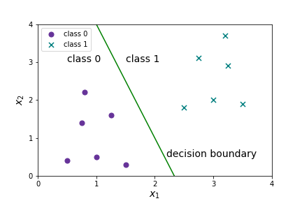
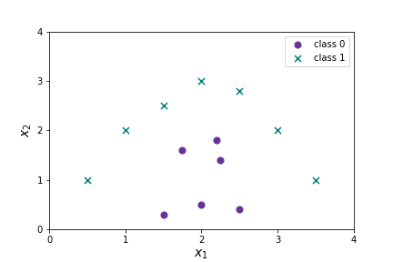
Note there is still a linear component to our model, so this will not work well for all data. Imagine the following data set:
Subsection 4.10 Logistic Regression Implementation
The sklearn code for implementing logistic regression should be easy to guess by now.
from sklearn.linear_model import LogisticRegression
log_reg = LogisticRegression(solver='lbfgs')
log_reg.fit(X_train, y_train)
log_reg.predict(X_test)
log_reg.score(X_test,y_test)
As usual the .fit creates the model for logistic regression, .predict applies the model, and .score returns the accuracy of the model. The attributes log_reg.intercept_ log_reg.coef_ give the intercept and slope for the linear decision boundary.
The main thing we haven't talked about yet is the solver='lbfgs'. The solver parameter is setting the type of optimization method to solve for \(\Theta\text{.}\) At present, “lbfgs” is recommended as the default, but the best choice will depend on data (especially size, but also other features such as sparsity). The five current options are listed below.
-
newton-cgNewton-cg is like gradient descent but uses information about first and second partial derivatives. Calculating the Hessian matrix (all the second order partial derivatives) is slow, and this method can land at saddle points instead of minimums.
-
lbfgsStands for Limited-memory Broyden–Fletcher–Goldfarb–Shanno. It approximates the second derivative matrix updates with gradient evaluations. It stores only the last few updates, so it saves memory. It isn't super fast with large data sets. Current default solver.
-
liblinearStands for Library for Large Linear Classification. Uses a coordinate descent algorithm. Coordinate descent is based on minimizing a multivariate function by solving one dimension at a time. Former default solver for Scikit-learn. It performs pretty well with high dimensionality. It does have a number of drawbacks. It can get stuck, is unable to run in parallel, and can only solve multi-class logistic regression with one-vs.-rest.
-
sagStochastic Average Gradient descent. A variation of gradient descent and incremental aggregated gradient approaches that uses a random sample of previous gradient values. Fast for big datasets.
-
sagaExtension of sag that also allows for L1 regularization. Should generally train faster than sag.
These descriptions are mostly taken from https://towardsdatascience.com/dont-sweat-the-solver-stuff-aea7cddc3451
More details can be found at https://stackoverflow.com/questions/38640109/logistic-regression-python-solvers-defintions/52388406#52388406
For our purposes, the default solver will be fine and our data sets aren't so complicated that we will need to explore different solvers. But in actual implementation you would want to examine different solvers based on on your data set and see which is most effective. There are also a number of hyperparameters related to each type of solver.
Let's do logistic regression on our super simple data set and see how well it matches our made-up line!
Hmmm. Our made-up line is a little flatter. Compare to Figure 4.16
So we just used LogisticRegression with all the default settings. What hyperparameters does it have?
LogisticRegression(C=1.0, class_weight=None, dual=False, fit_intercept=True,
                   intercept_scaling=1, l1_ratio=None, max_iter=100,
                   multi_class='auto', n_jobs=None, penalty='l2',
                   random_state=None, solver='lbfgs', tol=0.0001, verbose=0,
                   warm_start=False)
We've discussed a few of these parameters, solver='lbfgs' is the type of optimization. fit_intercept=True is a model parameter, it indicates whether or not to allow a \(y\)-intercept.
The rest of the parameters fall under the following categories:
-
Liblinear solver specific parameters
dual=Falseandintercept_scaling=1are only used for liblinear solver. -
Class related Parameters
class_weight=NoneShould there be a weighting based on the frequency of each class in the data set?multi_class='auto'This specifies how we should deal with more than two classes. The options are one-versus-rest and multinomial. We will discuss these in the next section! -
Stopping and Starting Conditions.
tol=.001andmax_iter=1000are stopping conditions.warm_start=FalseIndicates whether or not to reuse the solution of the previous call to fit as initialization. -
Regularization Parameters. The regularizer is a penalty added to the loss function that shrinks model parameters of \(\Theta\) towards the zero vector. We'll talk more about regularization later. These parameters include
C=1.0, l1_ratio=None, penalty='l2'. -
Processing Parameters.
random_state=NoneSets a random seed for reproducible outcomes.verbose=0Can print out lots of information as it runs through the iterations. Useful for debugging and evaluating code/model.n_jobs=NoneA parameter for parallelizing code.
Subsection 4.11 Multiclass logistic regression
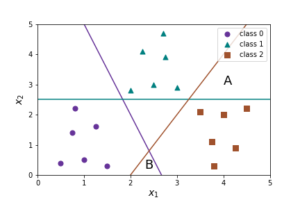
What should we do if we have more than two classes? There are two options for multi-class logistic regression: one-vs-rest (also called one-versus-all ) or multinomial. We will begin with one-vs-rest multi-class logistic regression. In this case we make no changes to our model we just apply it \(K\) where \(K\) is the number of classes. Suppose we have three classes
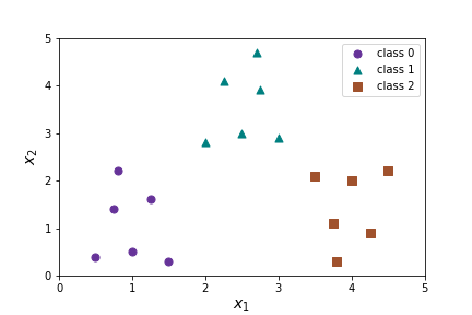
- Separate circles from everything else with \(h_\Theta^0(X)\)
- Separate triangles from everything else with \(h_\Theta^1(X)\)
- Separate squares from everything else with \(h_\Theta^2(X)\)
Then we predict the class of \(X\) by finding the max(\(h_\Theta^0(X)\text{,}\) \(h_\Theta^1(X)\text{,}\) \(h_\Theta^2(X)\)). As before this will produce linear decision boundaries, but it will produce three different linear decision boundaries.
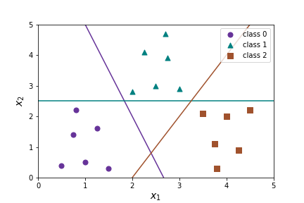
Activity 4.1.
Answer the following questions about the predictions \(h_\Theta^0(X)=P(y=\text{ class }0)\text{,}\) \(h_\Theta^1(X)=P(y=\text{ class }1)\text{,}\) \(h_\Theta^2(X)==P(y=\text{ class }2)\text{.}\)
- Suppose \(h_\Theta^0(X)=.6\text{,}\) \(h_\Theta^1(X)=.7\text{,}\) \(h_\Theta^2(X)=.3\text{.}\) What class will one-versus-rest predict for \(X\text{?}\) Approximately where on the graph will \(X\) be?
- Repeat the above problem for \(h_\Theta^0(X)=.3\text{,}\) \(h_\Theta^1(X)=.4\text{,}\) \(h_\Theta^2(X)=.8\text{.}\)
- Repeat the above problem for \(h_\Theta^0(X)=.5\text{,}\) \(h_\Theta^1(X)=.4\text{,}\) \(h_\Theta^2(X)=.4\text{.}\)
- Consider the points A,B on the graph. What can you say about the values of \(h_\Theta^0(X)\text{,}\) \(h_\Theta^1(X)\text{,}\) \(h_\Theta^2(X)\) at A? at B?
There is also a multinomial version of logistic regression that uses cross-entropy loss. In this case we change our model so can apply logistic regression for each class all at the same time.
-
Data: Add one-hot encoding for \(y\)
Identify features and labels in the data. Features are encapsulated in the \(m \times (f+1)\) matrix, \(X\text{,}\) and labels in the \(m \times 1\) matrix, \(y\) where the values in \(y\) occur in a discrete range, so far we have only discussed \(y_i \in \{0,1\}.\) To allow for the \(K\) classes we use a one one-hot encoding for \(y^i\text{.}\) That is, \(y^i\) is a \(K\) long vector, where all entries are 0 except for the \(y^i_k\) where \(X^i\) has class \(k\text{.}\) \(X\) remains the same.
\begin{equation*} X= \left[ \begin{matrix} 1 \amp x_1^{(1)} \amp x_2^{(1)} \amp x_3^{(1)}\amp \cdots \amp x_f^{(1)}\\ 1 \amp x_1^{(2)} \amp x_2^{(2)} \amp x_3^{(2)}\amp \cdots \amp x_f^{(2)}\\ \amp \amp \amp \vdots \amp \amp \\ 1 \amp x_1^{(m)} \amp x_2^{(m)} \amp x_3^{(m)}\amp \cdots \amp x_f^{(m)}\\ \end{matrix} \right] \end{equation*}and
\begin{equation*} y= \left[ \begin{matrix} 1 \amp 0 \amp 0 \amp 0 \cdots \amp 0\\ 0 \amp 0 \amp 0 \amp 1 \cdots \amp 0\\ \vdots \\ 0 \amp 0 \amp 1 \amp 0 \cdots \amp 0\\ \end{matrix} \right] = \left[ \begin{matrix} y^0 _1 \amp y^0 _2 \cdots \amp y^0 _K\\ y^1 _1 \amp y^1 _2 \cdots \amp y^1 _K\\ \vdots \\ y^m _1 \amp y^m _2 \cdots \amp y^m _K\\ \end{matrix} \right] \end{equation*} -
Learn Function.
Learn a function \(F\) such that \(F(X) \approx y \text{.}\) This is still the same.
-
Model: Softmax/Linear Model
In order to encode different information for each class we expand \(\Theta\) from a \(f+1 \times 1 \) matrix to a \(f+1 \times K \) matrix where each column \(\Theta^k\) corresponds to a model for the \(k\)th class.
\begin{equation*} \Theta = \left[ \begin{matrix} \theta_0^1 \amp \theta_0^2 \amp \theta_0^3 \amp \cdots \amp \theta_0^K\\ \theta_1^1 \amp \theta_1^2 \amp \theta_1^3 \amp \cdots \amp \theta_1^K\\ \vdots \\ \theta_f^1 \amp \theta_f^2 \amp \theta_f^3 \amp \cdots \amp \theta_f^K\\ \end{matrix} \right] \end{equation*}We still model the function with a combination of a linear and sigmoidal (S-shaped) function, but we use the softmax function \(\sigma\) instead of the logistic function. We define a model for each different class \(k\text{.}\)
\begin{equation*} h_{\Theta}(X^i)^k=\sigma(X^i,\Theta)^k =\frac{e^{X^i\theta^k}}{\sum_{j=1}^K e^{X^i\theta^j}} \end{equation*}This notation is somewhat cumbersome so we will switch to the book's notation here and use \(p_k\) instead of \(h_\Theta\text{.}\) That is, the model for the \(k\)th class is given by
\begin{equation*} \hat{p}_k(X^{(i)})=\frac{e^{X^i\theta^k}}{\sum_{j=1}^K e^{X^i\theta^j}}. \end{equation*}Remember we interpret this as the probability that \(X^{(i)}\) belongs to class \(k\text{.}\) Now, we have a \(k\) dimensional model, that is Thus, \(\hat{p}(X^{(i)})\) can be thought of as vector of length \(K\text{.}\)
\begin{equation*} \hat{p}(X^{(i)})=(\hat{p}_1(X^{(i)}), \hat{p}_2(X^{(i)}), \cdots \hat{p}_K(X^{(i)})). \end{equation*}Question 4.17.
How does this compare to the sigmoid/logistic function from before? AnswerIts similar; we can think of it as a generalization to more dimensions. From before we have:\begin{equation*} h_\Theta(X)=g({X}{\Theta})= \frac{1}{1+e^{-{X}{\Theta}}}. \end{equation*}Now we have\begin{equation*} \hat{p}_k(X^{(i)})=\frac{e^{X^i\theta^k}}{\sum_{j=1}^K e^{X^i\theta^j}}\\ = \frac{e^{X^i\theta^k}}{e^{X^i\theta^1}+e^{X^i\theta^2}+ \cdots +e^{X^i\theta^K} } \end{equation*}\begin{equation*} = \frac{1} {e^{-X^i\theta^k} \left( e^{X^i\theta^1}+e^{X^i\theta^2}+ \cdots +e^{X^i\theta^K}\right) } \end{equation*}\begin{equation*} = \frac{1} {1+e^{-X^i\theta^k} \sum_{j\neq k}^K e^{X^i\theta^j}} \end{equation*}Question 4.18.
What's the smallest possible value for \(\hat{p}_k(X^{(i)})\text{?}\) When will it reach that value? What's the largest \(\hat{p}_k(X^{(i)})\text{?}\) When will it reach that value? What's the desired value of \(\hat{p}_k(X^{(i)})\text{?}\)
AnswerSince
\begin{equation*} \hat{p}_k(X^{(i)}) = \frac{1} {1+e^{-X^i\theta^k} \sum_{j\neq k}^K e^{X^i\theta^j}} \end{equation*}and
\begin{equation*} 0 \leq e^{-X^i\theta^k} \sum_{j\neq k}^K e^{X^i\theta^j} \lt \infty \end{equation*}then the smallest value is \(\hat{p}_k(X^{(i)})\approx 0 \) when \(e^{-X^i\theta^k} \sum_{j\neq k}^K e^{X^i\theta^j} \to \infty \text{.}\)
The largest value is \(\hat{p}_k(X^{(i)})=1\) when \(e^{-X^i\theta^k} \sum_{j\neq k}^K e^{X^i\theta^j} = 0 \text{.}\)
Whew! Why whew? Hint
We did say we are thinking of it as a probability after all.The desired value of \(\hat{p}_k(X^{(i)})\) depends on the class of \(X^{(i)}\text{.}\) We hope it is near one if \(X^{(i)}\) has class \(k\) and near zero if \((X^{(i)})\) does not have class \(k\text{.}\) That is, if \(X^{(i)}\) has class \(k\) then we hope
\begin{equation*} \hat{p}_k(X^{(i)}) \approx 1 \\ \text{ and } \hat{p}_j(X^{(i)}) \approx 0 \text{ for } j \neq k \end{equation*} -
Cost Function: Cross Entropy Loss
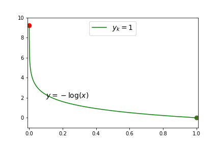
We will change the cost function to the cross entropy loss function. Cross entropy is a term from information theory and the idea is that the cost should be high if the model predicts a low probability for the target class, and the cost should be low if the model predicts a high probability for the target class. (Similar to the log-loss function.) For \(K\) classes
\begin{equation*} J = -\frac{1}{m} \sum_{i=1} ^m \sum_{j=1} ^K y_j ^{(i)} \log( \hat{p}_j(X^{(i)})). \end{equation*}If \(y^i\) is the ith row of the y matrix, \(y^i=( y_1^i, y_2^i, \cdots, y_K^i) \) and \(g^i=\log(\hat{p}_k(X^{(i)})=(\log(\hat{p}_1(X^{(i)})), \log(\hat{p}_2(X^{(i)})), \cdots \log(\hat{p}_K(X^{(i)})))\) then we can represent \(J\) using a dot product,
\begin{equation*} J = -\frac{1}{m} \sum_{i=1} ^m \sum_{j=1} ^K y^i \cdotp g^i\text{.} \end{equation*}Question 4.19.
What is the shape of J? Answer\(1 \times 1\text{!}\) Yay! Its a number.Question 4.20.
How many nonzero terms in \(\sum_{j=1} ^K y_j ^{(i)} \log( \hat{p}_j(X^{(i)}))\) for a fixed \(X^{(i)}\text{?}\) AnswerRemember that we one-hot encoded \(y^i\) so that it is all zeros except in the \(k\)th position where \(k\) is the class of \(X^i\text{.}\) Thus \(\sum_{j=1} ^K y^i \cdotp g^i\) contains only one non-zero entry, namely \(y_k ^{(i)} \log( \hat{p}_k(X^{(i)})) = \log( \hat{p}_k(X^{(i)}))\text{!}\) [Since \(y_k ^{(i)}=1\text{.}\)] Thus the cost function only cares about the probability function that corresponds to the class of \(X^{(i)}\text{,}\) \(\hat{p}_k(X^{(i)})\text{,}\) and doesn't care about the probability functions that do not correspond to the class of \(X^{(i)}\text{,}\) \(\hat{p}_j(X^{(i)})\) where \(j \neq k\text{.}\)Question 4.21.
How does this compare to the log-loss function we used before? AnswerIts similar. Its really just a generalization to higher dimensions! And with a slight modification (simplification!) because of the one-hot encoding for \(y\text{.}\) Before we had\begin{equation*} J = -\frac{1}{m} \sum_{i=1} ^m y_i\log(h_\Theta(X^{(i)})) +(1-y_i)\log(1-h_\Theta(X{(i)})) \text{.} \end{equation*}We had to fuss with the \(y_i\) vs \(1-y_i\) and \(-\log(h_\Theta)\) vs \(-\log(1-h_\Theta)\) because if the class was zero and we predicted zero we want a low cost, but if the class was one and we predicted one we also want a low cost.In our new model, if the class is correct we always want to get one because we have one-hot encoded our data rather than trying to get out the value of the class. So we just want the sum over the \(y_i\log(h_\Theta(X^{(i)}))\) pieces.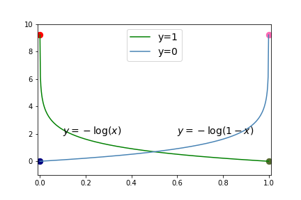
-
Optimization Technique.
Same as before, we want to use the most appropriate optimization technique for our data set.
-
Make Predictions!
We still interpret \(\hat{p}_k(X^{(i)})\) as the probability that \(X^i\) has class \(k\) given \(X^i\) and \(\Theta\text{.}\) However, we have \(K\) classes, and \(K\) different \(\hat{p}_j(X^{(i)})\) functions, so we can no longer use the threshold method to predict a specific class rather than a probability. But we already solved this for our other multi-class system! Instead, we pick the class with the largest probability score. We predict a class by
\begin{equation*} \operatorname{argmax}_k \hat{p}_k(X^{(i)}). \end{equation*}The function argmax returns the value \(k\) with the largest \(\hat{p}_k(X^{(i)})\text{.}\)
Question 4.22.
Whew! That's quite a model. One-versus-all seems much easier. Why do we need multinomial? Why did we spend so much time on logistic regression?? Answer
Time for a Jupyter notebook!
https://colab.research.google.com/drive/1D1ZCIdRszI3igx43K5qJ4KNW6fGitfhS?usp=sharingSubsection 4.12 Notes from Exam 1
Question 4.23.
What is the difference between StandardScaler(), MinMaxScaler(), LinearRegression(normalize=True)? When do we use each one? Which ones have only positive values? Which one is best for data with outliers?
Here are histograms for the mass data from the fruit data set in Exam 1 with each of the different techniques applied.
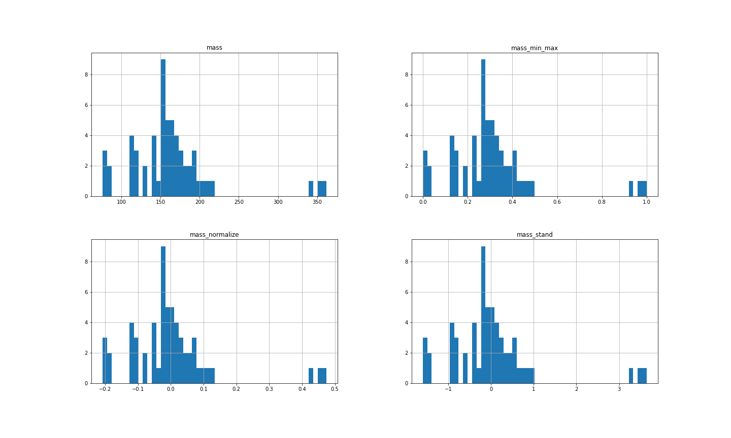
| scaling technique | mean | standard deviation | min | max |
| NONE | 163.12 | 55.02 | 76 | 362 |
| StandardScaler() | 0 | 1.01 | -1.60 | 3.65 |
| MinMaxScaler | 0.30 | 0.19 | 0 | 1 |
| normalize=True | 0 | 0.13 | -0.21 | 0.47 |
The formula for StandardScaler() is
The purpose of this type of feature scaling is to center the data around 0, and have variance =1. (Remember variance = (standard deviation)\(^2\text{.}\))
The formula for MinMaxScaler() is
The purpose of this type of feature scaling is to scale the data into the interval \([0, 1] \text{.}\) (If \(x=\min(x)\) then \({\frac {x-\min(x)}{\max(x)-\min(x)}}=0\) and if \(x=\max(x)\) then \({\frac {x-\min(x)}{\max(x)-\min(x)}}=1\text{.}\))
The formula for normalize=True is
In this case, \(\|x-\operatorname{mean}(x)\|^2\) is the Euclidean distance (l2-norm) between \(x\) and \(\operatorname{mean}(x)\text{.}\) That is,
The purpose of this type of feature scaling is center the data around 0, so that the sum of the l2 norms of all data points is equal to 1. In this case,
and
Question 4.24.
So which was best for outliers?
AnswerNONE OF THEM! Scaling does not help with outliers! Scaling changes the range of values, but it preserves the relationships between points. Scaling helps optimization parameters, it doesn't help cleaning up our data.
The code for the last question is here in case you are interested.
Question 4.25.
What happens if we skip the plt.show()? Answer
 array([[< matplotlib.axes._subplots.AxesSubplot object at 0x7f99e0d290d0>,
        < matplotlib.axes._subplots.AxesSubplot object at 0x7f99e1963890>],
       [< matplotlib.axes._subplots.AxesSubplot object at 0x7f99e0d6ed10>,
        < matplotlib.axes._subplots.AxesSubplot object at 0x7f99e15f8550>]],
      dtype=object)
Its not as pretty! Please use plt.show()!
Question 4.26.
What should we do with outliers? Answer
Here are three different ways that feature scaling could interact with training and testing. What are the differences in these three techniques? Which is best and why? Option 1 Option 2 Option 3 Option 1 is problematic because you are secretly leaking information about the testing set to your model since the parameters by which to scale the data include the testing data. Your model may no longer work as well when applied to different data. Remember the goal of the testing data is to keep it completely separate from building your model. You want to see how your model is going to perform on data that it has no information about it. Option 2 is problematic because your model is only designed to work based on the scaling applied on the training data. The testing data may have completely different parameters. So your model may perform poorly on the testing data. Option 3 is the best! We do not refit on testing data. We just apply the transformation from training data. So the model should work well on the testing data. We also have not secretly leaked any information about our model so it should perform similarly on new data.
Question 4.27.
Answer
Note that the mean and standard deviation for the entire data set is not the same as for just the training set alone. The model is secretly cheating and getting information about the testing set!!
Also note how different the scores are between the training and the testing set. The command scaler.fit_transform() will do something very different on each of these sets. We don't want that. We need to do the exactly same operations on the testing set that we did to the training set.
Yeah, but this was the random split. This won't be so bad for the stratified split. Right?

So be careful about the connection between scaling and train/test/split! In general, never call .fit on your testing set. Any command involving .fit is part of building the model and the model should not have any information about the testing set.