
Section 1 k Nearest Neighbors
Our first machine learning algorithm! In general the goal of a machine learning algorithm is to learn a function
that can predict the values \(y\) for a data point \(\vec{x}\) after training on a large data set \(\vec{X}\text{.}\) The values of \(y\) might be discrete for predicting a class (e.g., the type of iris), or continuous for predicting a value (e.g., the price of a house). Our first machine learning algorithm is \(k\) Nearest Neighbors (called kNN for short).
kNN is a supervised learning algorithm that can be used for either classification (discrete) or regresssion (continuous). It is an instance or memory based algorithm. Essentially, this means that the algorithm memorizes the training data set and uses those memorized examples to make a determination for new objects. The variable \(k\) refers to the number of nearest neighbors to use.
Subsection 1.1 kNN for Classification
So how does kNN work for classification?
For classification, to determine the class of a new point, the algorithm examines the training data and finds the nearest \(k\) points. It uses the labels of those points to determine the label of the new point. There are a number of parameters to consider when implementing kNN.
What does nearest mean? We need to specify a distance metric. Euclidean distance is the default metric here, but others may be used.
How is the label of the new point determined? Again, there are multiple options. The default option is to use a majority vote where each point is weighted equally. A different option would be to weight points by their distance to the point we are attempting to label.
And, of course, there is \(k\)! How many nearest neighbors should be used? The default is 5, but this should be determined from the situation or the specific data. Majority vote will not work well if \(k\) is even, so generally we only consider odd \(k\text{.}\) It also doesn't make sense to use more points than we have, so \(k\) must be less than the total number of points.
We begin with a very small example to illustrate the concept. This data set has only three points and, of course, is way too small to really apply machine learning techniques. Each data point has two features and a classification which is either 0 or 1.
| Datapoint | \(X_1\) feature | \(X_2\) feature | Class |
| A | \(2\) | \(3\) | 1 |
| B | \(4\) | \(1\) | 0 |
| C | \(5\) | \(5\) | 0 |
To see how kNN works, we want to classify a new point \((4,2)\) as either 0 or 1. How should we do this?
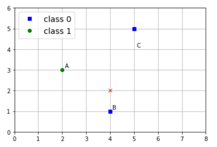
We will use Euclidean distance and majority vote with uniform weights. We have two options for an odd \(k\text{:}\) either 1 or 3. (Why are these the only two?) We'll apply both.
We first need to calculate the (Euclidean) distance between the points in our data set and \((4,2)\text{.}\)
| Datapoint | Distance to (4,2) | Class |
| A | \(\sqrt{5}\) | 1 |
| B | \(1\) | 0 |
| C | \(\sqrt{10}\) | 0 |
For \(k=1\text{,}\) \(B\) is the closest point to \((4,2)\text{.}\) It has class 0, so we assign the class of 0 to point \((4,2)\text{.}\)
For \(k=3\text{,}\) the three nearest points are all the data points in our set. Thus, we do a majority vote of all three data points, which also gives a class of 0.
Question 1.3.
What classification will be assigned to the points \((1,3), (6,3), (2,1) \) with \(k=1\text{?}\) with \(k=3\text{?}\)
AnswerSubsection 1.2 kNN for Regression
So how does \(kNN\) work for regression?
In this case, we want to predict the \(y\) value instead of a classification. To do this, compute the nearest \(k\) points and average their \(y\) values. Note, we are not applying majority rule, so even values of \(k\) make sense for regression.
We will consider the same very small data set of 3 data points. Each data point has an \(x_1\) value, an \(x_2\) value, and a \(y\) value. (We could think of these as points in 3D, with \((x,y,z)\) coordinates.) We want to predict a \(y\) value for new points, based on the nearest points.
| Datapoint | \(X_1\) feature | \(X_2\) feature | \(Y\) feature |
| A | \(2\) | \(3\) | \(4\) |
| B | \(4\) | \(1\) | \(7\) |
| C | \(5\) | \(5\) | \(6\) |
How should we predict the \(y\) value for \((x_1,x_2)=(4,2)\text{?}\) Now we have three options for \(k\text{:}\) 1,2 or 3.
From Table 1.2, we see that point \(B\) is closest, followed by point \(A\text{,}\) and then by point \(C\text{.}\) Thus the predicted \(y\) value for \(k=1\) is 7. For \(k=2\text{,}\) it is \(\frac{1}{2}(4+7)=5.5\text{.}\) For \(k=3\text{,}\) it is \(\frac{1}{3}(4+7+6)=\frac{17}{3}\text{.}\)
Question 1.5.
What \(y\) value will \(k\)NN predict for points \((1,3), (6,3), (2,1) \) with \(k=1\text{?}\) with \(k=2\text{?}\) with \(k=3\text{?}\)
AnswerSubsection 1.3 Simple Implementation of kNN
We will begin with a python implementation of our super tiny examples from Table 1.1 and Table 1.4. We first enter our data set in both numpy and pandas formats, and graph our points.
We now are ready to apply kNN for classification! We will again take advantage of sklearn. We first import with
from sklearn.neighbors import KNeighborsClassifier
and then instantiate with
knn = KNeighborsClassifier(n_neighbors = 1)
.
We can then apply attributes for knn. The main attributes are:
-
knn.fit(X, y)Fit the model using \(X\) as training data and \(y\) as target values (labels). \(X\) is array-like with shape (number of samples, number of features). \(y\) is array-like with shape (number of samples,) or (number of samples, number of outputs). -
knn.predict(X)Predict the class labels for the provided data. \(X\) is array-like of inputs with shape (number of samples, number of features). -
knn.score(X,y)Return the mean accuracy on the given test data and labels. \(X\) and \(y\) as in knn.fit(X,y).
Note: array-like means we can enter data as either numpy array or pandas dataframe.
Hooray! We did our first tiny example of using kNN for classification!
What should we change for our tiny example of using knn for Regression?
There are many kNN parameters that we can explore!
-
n_neighbors: Number of neighbors to use, default =5 -
weights: how to weight points (equally or by distance or custom), default = 'uniform' weight function used in prediction. Possible values: -
algorithm: Algorithm used to find the nearest neighbors {'auto', 'ball_tree', 'kd_tree', 'brute'}, default='auto' -
leaf_size: Leaf size passed to BallTree or KDTree, default = 30. -
metric: the distance metric to use for the tree, default 'minkowski'\begin{equation*} {\displaystyle D\left(X,Y\right)=\left(\sum _{i=1}^{n}|x_{i}-y_{i}|^{p}\right)^{\frac {1}{p}}} \end{equation*} -
p: Power parameter for the Minkowski metric, default = 2. -
metric_params: Additional keyword arguments for the metric function, default = None -
n_jobs: The number of parallel jobs to run for neighbors search, default=None
Question 1.6.
These parameters should bring up some questions!
-
What is the Minkowski metric for \(p=1,2\text{?}\)
AnswerThe Minkowski metric for \(p=1\)
\begin{equation*} D\left(X,Y\right)=\left(\sum _{i=1}^{n}|x_{i}-y_{i}|\right). \end{equation*}(Taxi-cab metric.)
The Minkowski metric for \(p=2\)
\begin{equation*} D\left(X,Y\right) =\left(\sum _{i=1}^{n}|x_{i}-y_{i}|^{2}\right)^{\frac {1}{2}} =\sqrt{ \sum _{i=1}^{n}(x_{i}-y_{i})^{2}} \end{equation*}(Euclidean Metric)
-
Any sense from these parameters about what the computational challenges for kNN are?
AnswerFinding the \(k\) nearest neighbors is computationally intensive when the data set is large. In the worst case scenario, all distances must be computed between a test point and each point in the data set. Then these distances must be sorted. (And repeated for each new test point!) The algorithms give us some indication that there are more efficient ways to do this than what I just described.
-
Are large values of \(k\) or small values of \(k\) better?
AnswerTrick question! Neither both really small and really large values are equally bad. Note that large values of \(k\) don't provide much ability to distinguish points. In the worst case example, for classification with \(k=\) the number of points in the data set, knn always predicts the same value for all test points (the class that occurs most in the data set). This is called underfitting. We are under-using the information provided by the training data. (We will not make good predictions on either the training set or the testing set.) For really small values of \(k\) we are overfitting the data set. We are over-using the information provided by the training data. (We can predict the training set well (maybe even exactly), but won't predict well on the testing set.) What we want is to find the value of \(k\) that strikes the perfect balance between overfitting and underfitting (where we make good predictions on both the training and testing set). This theme of finding the “just right” fit is one that will come up in all of our machine learning algorithms.
Subsection 1.4 Visualizing Decision Boundaries
For classification, we often want to visualize the decision boundary. To do this we want to apply knn.predict() to a large number of points in our \(x,y\) grid and use a contour map to differently color regions that correspond to a different classification.
Wait! What happened?
The idea is that we want to create a grid of \(x\) and \(y\) values and apply knn.predict on all of those values. The we use plt.contourf(x_val, y_val, z_val,1) to create a filled contour plot to color the points where class=1 with one color (green) and use a different color (blue) to shade in all the points where class=0.
-
x_valspecifies the \(m\) different values of \(x\) either as a 1D array, or as a 2D \(n \times m\) array which repeats the values of \(x\) in each row. -
y_valspecifies the \(n\) different values of \(y\) either as a 1D array, or as a 2D \(n \times m\) array which repeats the values of \(y\) in each column. - The
z_valshould be an \(n \times m\) array where the columns correspond to \(x\) values and the rows correspond to \(y\) values. (Does this seem backwards?)\begin{equation*} z_{val}= \left[ \begin{matrix} z(x_0,y_0) \amp z(x_1, y_0) \amp \cdots \amp z(x_m, y_0) \\ \vdots \amp \vdots \amp \vdots \amp \vdots \\ z(x_0,y_n) \amp z(x_1, y_n) \amp \cdots \amp z(x_m, y_n) \\ \end{matrix} \right]. \end{equation*} - In general, you can specify how many contours to draw and what colors to use. The 1 will create one boundary (i.e., draw two contours.) Or you can create a custom color map and tell it explicitly which colors to use.
To create a tiny example, suppose the \(x\) values are \(\{1,3,5\}\) and the \(y\) values are \(\{2,4\}\text{.}\) We will construct all the arrays as 2D \(2 \times 3\) arrays.
To create the decision boundaries for kNN we want
Unfortunately, knn.predict() doesn't automatically act on arrays of this shape, so we have to do a lot of reshaping/rearranging commands. We first create a \(6 \times 2\) array where each row is a \((x,y)\) point for input into knn.predict(). The output will be a \(6 \times 1\) array that then needs to be converted to \(2\times 3\) array.
Step 1: Specify \(x\) and \(y\) ranges and create \(2 \times 3\) arrays where
In general, this uses np.linspace() for creating ranges and np.meshgrid for expanding to \(n \times m\) arrays.
Step 2: Convert \(x_{val}\) and \(y_{val}\) into one \(6 \times 2\) array.
In general, this uses .ravel and np.c_ to first flatten to 1D arrays and then vertically stack 1D arrays into each column of a 2D array.
Step 3: Compute \(y_{predict}=\)>knn.predict\((X_{new})\) to get \(6 \times 1\)
knn.predict(x,y) |
knn.predict(1,2) |
knn.predict(3,2) |
knn.predict(5,2) |
knn.predict(1,4) |
knn.predict(3,4) |
knn.predict(5,4) |
Step 4: Reshape \(y_{predict}\) to get
Step 5: Create contour plot with plt.contourf(x_val, y_val, z_val,1)
Note: In the example for the Iris data set, we didn't specify the number of contours, but instead used a custom color map to both set the number of contours and specify the colors.
from matplotlib.colors import ListedColormap
custom_cmap = ListedColormap(['#a0faa0','#9898ff'])
plt.contourf(x0, y0, z0, cmap=custom_cmap)
Subsection 1.5 Implementation of kNN on Iris Data Set
But, of course, our tiny examples are way too small to really apply machine learning. Let's return to the Iris Data set and look at the implementation details for how to classify the three different kinds of Iris. We'll jump over to a Jupyter notebook in Colab.
https://colab.research.google.com/drive/1DueksfooF4FTPNOB8AjKRX1vJPrfeYTy?usp=sharing