Section 8 Clustering
We are finally getting another example of unsupervised learning!!! Remember that unsupervised learning involves giving unlabeled data to an algorithm and asking the algorithm to find some structure or patterns in the data. In our previous example of unsupervised learning, PCA, we constructed an algorithm to find the structure of a lower dimensional space in the data. For clustering, we want to construct an algorithm to group similar instances into clusters.
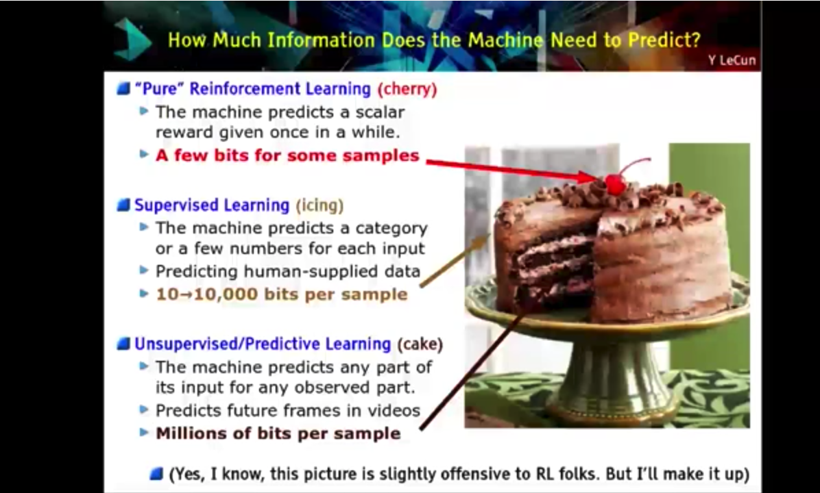
In this course, we are focusing primarily on supervised learning. Its the traditional starting place, and many of the most exciting current applications are based on these techniques. However, supervised learning requires labeled data. The vast majority of available data is unlabeled and labeling data is an expensive process because it almost always require human time to label the data. Facebook artificial intelligence Chief, Yann LeCun, gave a now famous analogy at NIPS 2016 (Conference on Neural Information Processing Systems).
If intelligence was a cake, unsupervised learning would be the cake, supervised learning would be the icing on the cake, and reinforcement learning would be the cherry on the cakeat NIPS 2016 (Conference on Neural Information Processing Systems). An image of one of his slides is below.
Clustering has a wide array of uses in data analysis. Examples include:
- Market Segmentation: Identify market segments to better design products to appeal to similar groups of customers.
- Anomaly Detection: Identify points that are far away from any cluster. Can be used to detect fraud or manufacturing defects.
- Search Engines: Identify similar pages/images/etc to return results for a search.
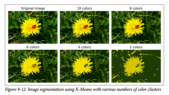
- Image Segmentation: Cluster pixels in an image according to their color to reduce the number of colors in an image. Often useful in detection and tracking systems.
- Data Analysis: One technique for data analysis on large data sets is to run a clustering algorithm and analyze each cluster separately.
- Social Network Analysis: Analyze clusters of friends.
- Data Center Analysis: Organize computer clusters/data centers based on which computers/servers talk to each other most frequently.
- Astronomical Data Analysis: Analyze the formation of galaxies.
- Semi-Supervised Learning: If you have data that you want labeled for supervised learning, but only have a small amount of labeled data, you can apply clustering and propagate the labels to all points in those clusters.
Subsection 8.1 K-means Clustering
There are many different clustering algorithms but we will focus on the K-means algorithm which is by far the most popular and widely used. K-Means is a simple, iterative algorithm that can cluster a dataset quickly and efficiently, often in just a few iterations. It was proposed by Stuart Lloyd at Bell Labs in 1957 as a technique for pulse-code modulation, but not published outside of the company until 1982. In 1965, Edward W. Forgy published a very similar algorithm.
The idea behind the K-means algorithm is a simple iterative process. The number of clusters, \(K\text{,}\) must be specified.
-
Step 1
- Assign a centroid for each of the \(K\) clusters randomly.
- Compute the distance between each point and each of the \(K\) centroids.
- Assign points to a cluster based on the nearest centroid. (There is a choice to make if there is a tie. We will assign these randomly.)
-
Step 2
- Assign a centroid for each of the \(K\) clusters by computing the mean value of all points in the cluster.
- Compute the distance between each point and each of the \(K\) centroids.
- Assign points to a cluster based on the nearest centroid.
Step 3 - Step \(n\text{.}\) Repeat step 2 until the centroids converge to a stable value.
Example 8.1.
Suppose we have a data set with two features and six points and we want to group the data into two clusters.
| \(x_1\) | \(x_2\) |
| 1.1 | 2.0 |
| 2.1 | 0.0 |
| 4.1 | 1.0 |
| 2.9 | 4.0 |
| 4.9 | 2.0 |
| 1.1 | 4.0 |
| 4.1 | 5.0 |
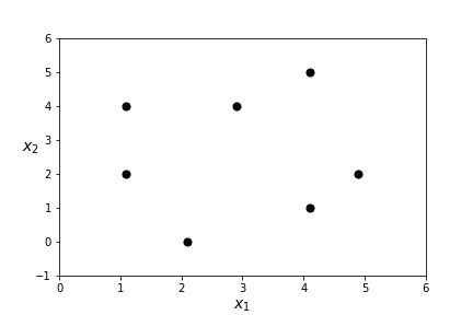
Question 8.2.
What two clusters do you see?Let's see what clusters K-means finds!
-
Step 1
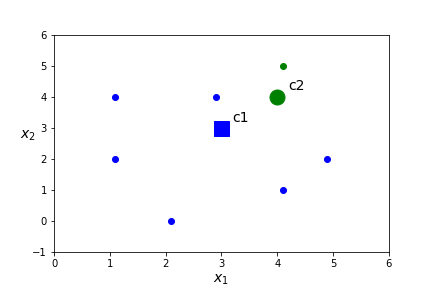
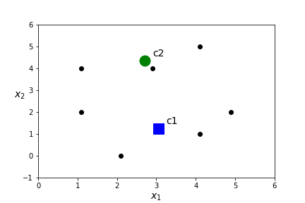
- Assign a centroid for each of the \(K\) clusters randomly. Pick \(c_1=(3,3)\) and \(c_1=(4,4)\)
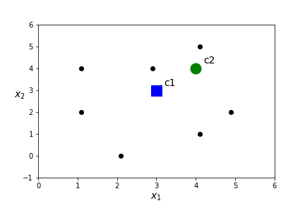
- Compute the distance between each point and each of the \(K\) centroids. Assign points to a cluster based on the nearest centroid.
\(x\) dist(x,c1) dist(x,c2) closest centroid (1.1,2.0) 2.15 3.52 c1 (2.1,0.0) 3.13 4.43 c1 (4.1,1.0) 2.28 3.00 c1 (2.9,4.0) 1.00 1.10 c1 (4.9,2.0) 2.15 2.19 c1 (1.1,4.0) 2.15 2.90 c1 (4.1,5.0) 2.28 1.00 c2 - Assign points to a cluster based on the nearest centroid.
- Assign a centroid for each of the \(K\) clusters randomly. Pick \(c_1=(3,3)\) and \(c_1=(4,4)\)
-
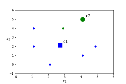
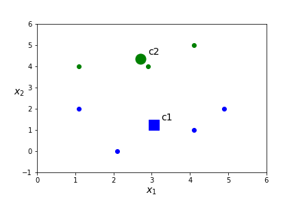
Step 2
- Assign a centroid for each of the \(K\) clusters by computing the mean value of all points in the cluster. In this case\begin{equation*} c_1=\frac{(1.1,2)+(2.1,0)+(4.1,1)+ (2.9,4)+(4.9,2)+(1.1,4)}{6}= (2.7,2.17) \end{equation*}\begin{equation*} c_2=(4.1,5). \end{equation*}

- Compute the distance between each point and each of the \(K\) centroids.
\(x\) dist(x,c1) dist(x,c2) closest centroid (1.1,2.0) 1.61 4.24 c1 (2.1,0.0) 2.25 5.39 c1 (4.1,1.0) 1.82 4.00 c1 (2.9,4.0) 1.84 1.56 c2 (4.9,2.0) 2.21 3.10 c1 (1.1,4.0) 2.43 3.16 c1 (4.1,5.0) 3.16 0.00 c2 - Assign points to a cluster based on the nearest centroid.
- Assign a centroid for each of the \(K\) clusters by computing the mean value of all points in the cluster. In this case
-
Step 3
- Assign a centroid for each of the \(K\) clusters by computing the mean value of all points in the cluster. In this case\begin{equation*} c_1=\frac{(1.1,2)+(2.1,0)+(4.1,1)+(4.9,2)+(1.1,4)}{5}= (2.66,1.8) \end{equation*}\begin{equation*} c_2=\frac{(4.1,5)+ (2.9,4)}{2}=(3.5,4.5). \end{equation*}
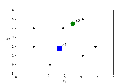
- Compute the distance between each point and each of the \(K\) centroids.
\(x\) dist(x,c1) dist(x,c2) closest centroid (1.1,2.0) 1.57 3.47 c1 (2.1,0.0) 1.89 4.71 c1 (4.1,1.0) 1.65 3.55 c1 (2.9,4.0) 2.21 0.78 c2 (4.9,2.0) 2.25 2.87 c1 (1.1,4.0) 2.70 2.45 c2 (4.1,5.0) 3.51 0.78 c2 - Assign points to a cluster based on the nearest centroid.
- Assign a centroid for each of the \(K\) clusters by computing the mean value of all points in the cluster. In this case
-
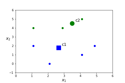
Step 4
- Assign a centroid for each of the \(K\) clusters by computing the mean value of all points in the cluster. In this case\begin{equation*} c_1=\frac{(1.1,2)+(2.1,0)+(4.1,1)+(4.9,2)}{4}= (3.05,1.25) \end{equation*}\begin{equation*} c_2=\frac{(4.1,5)+ (2.9,4)+(1.1,4)}{3}=(2.7,4.33). \end{equation*}
- Compute the distance between each point and each of the \(K\) centroids.
\(x\) dist(x,c1) dist(x,c2) closest centroid (1.1,2.0) 2.09 2.83 c1 (2.1,0.0) 1.57 4.37 c1 (4.1,1.0) 1.08 3.62 c1 (2.9,4.0) 2.75 0.39 c2 (4.9,2.0) 2.00 3.21 c1 (1.1,4.0) 3.37 1.63 c2 (4.1,5.0) 3.89 1.55 c2 - Assign points to a cluster based on the nearest centroid.
- Assign a centroid for each of the \(K\) clusters by computing the mean value of all points in the cluster. In this case
Question 8.3.
What will happen in Step 5? Answer
Question 8.4.
What do you think of the clusters K-means found? Answer
Question 8.5.
What do you think happens if we start with different initial centroids? Answer
cent=np.array([[0,2],[5,2]]) or cent=np.array([[0,0],[4,4]])
We can see in the code that it is easy to use sklearn to invoke KMeans. We need
from sklearn.cluster import KMeans
kmeans=KMeans(n_clusters=2,init=cent,n_init=1)
The full list of parameters are
KMeans(algorithm='auto', copy_x=True, init='k-means++', max_iter=300,
       n_clusters=8, n_init=10, n_jobs=None, precompute_distances='auto',
       random_state=None, tol=0.0001, verbose=0)
The main parameter to explore is n_clusters. In some cases there is an obvious number of clusters based on the purpose of the model, but usually this is something we want to explore.
n_init=10 is the number of times the program will be run with different randomly chosen initial centers. As we have seen, this is quite important as KMeans is very sensitive to this initial choice of centers.
There are a few optimizations for KMeans that we will discuss in the next section. There are better strategies for picking initial centers other than picking random centers. (This corresponds to the init parameter.) It can be a lot of work to compute all the distances and there are some optimizations of that process related to choices in algorithm and precompute_distances.
Important attribues already used in the above code are
cluster_centers_ and
labels_ .
Question 8.6.
Below are four of the different clusters that are possible based on different initial centroids. Which one do you think is best? What should best mean? 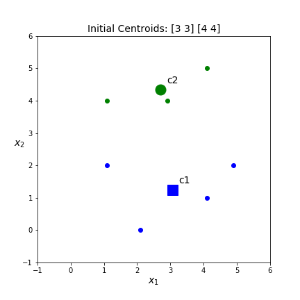
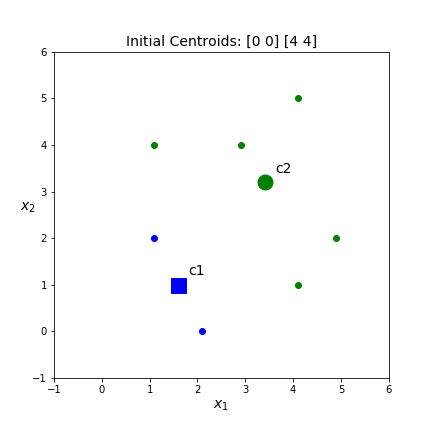
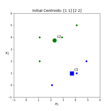
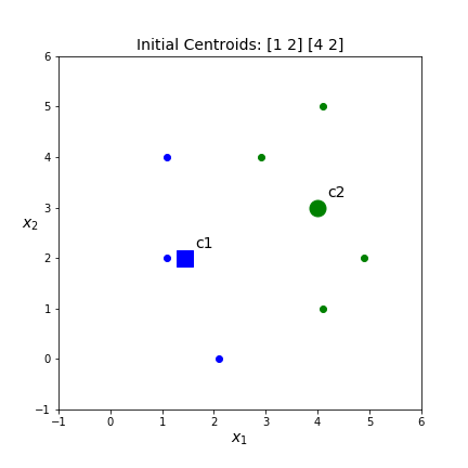
kmeans.inertia_ . This is the score KMeans uses to determine which of the different sets of clusters is best. The inertia scores for the above clusters are 17.21, 22.07, 17.39, 20.71 respectively. Thus, the top left set of clusters is the best. However, both left hand sets of clusters are pretty similar.
Subsection 8.2 Optimizing KMeans
The optimization objective in KMeans clustering is to minimize the sum of squared distances between each point and its closest centroid. To write this as a formula let \(c_j\) denote the \(j\)th cluster centroid. (In sklearn, kmeans.cluster_centers_[j].) Let \(L_i \) denote the index of the cluster that \(x^i\) is assigned to (In sklearn, kmeans.labels_[i].) Then the cluster centroid that is closest to \(x^i\) is given by \(c_{L_i}\text{.}\) (In sklearn, kmeans.cluster_centers_[kmeans.labels_[i]]). Thus our optimization objective \(J\) is a function of both the centroids and the cluster assignments and is given by
(In sklearn, kmeans.inertia_).
Essentially we have two steps that we alternate between Step A: For fixed centroids, assign points to a cluster based on the closest centroid. This assignment of points will minimize the sum of squared distances between points and a fixed set of centroids. (Minimizes J as we vary cluster assignment, but fix centroids.) Step B: For fixed cluster assignments, change the centroid to the mean of all points in the cluster. This is the location that will minimize the sum of distances between points and centroid for a fixed cluster assignment. (Minimizes \(J\) as we vary centroids, but fix cluster assignment.) Alternating between these two steps will minimize \(J\) relative to both centroids and cluster assignments.
Question 8.7.
How do the steps in KMeans clustering optimize this function? Answer
Question 8.8.
What should happen to \(J\) as we iterate the algorithm for a fixed number of clusters? Can \(J\) ever increase? Can \(J\) remain constant? Answer
Question 8.9.
What should happen to \(J\) as we increase the number of clusters \(K\text{?}\) Can \(J\) ever increase? Can \(J\) remain constant? Could \(J=0\text{?}\) Answer
We've seen how much impact the starting choice of centroids can have to the final set of clusters. It is entirely possible that this algorithm can get stuck at local minimum for \(J\text{.}\) One solution is choose multiple different random initializers and keep the one with the lowest cost. The default option is to choose ten different initial centroids. But there are some other options that will help the algorithm converge more quickly. n_init=10
Question 8.10.
Should we ever pick two initial centroids to be the same? What about just close? Answer
Here are three options for picking initial centroids:
- Pick \(k\) random centroids. We did this in the example, but it isn't recommended in practice.
- Pick k distinct points from the data set. (Randomly, but points are chosen randomly from data set rather than randomly from a given distribution.)
init='random'implements this choice. - Pick one centroid at random from the data set. Then picks the next according to a probability distribution which encourages the next centroid to be far away from the centroids selected so far.
init='k-means++'is the default setting.
How should we choose the number of clusters?
- There may be a goal of your data set that specifies the best number of clusters. You want to design T-shirts and will have 3 sizes, small, medium, large. You can identify three clusters of clothing proportions in your data.
- In many cases, there is not a right answer.
- One technique is to apply the "elbow technique". Plot J versus the number of clusters. J will keep decreasing as K increases, but there may be an "elbow" where it appears increasing L does not result in a substantial lowering of J.
Much of the work in KMeans involves computing distances. This can get computationally overwhelming. There is a technique called the Elkan technique which uses the triangle inequality to keep track of lower and upper bounds for distances between points and centroids. Whether to use the Elkan technique or not, really depends on the type of data you have. It does not support sparse data. However algorithm='auto' will take care of making this decision for you.
Question 8.11.
What is the triangle inequality? Answer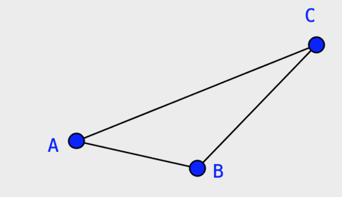
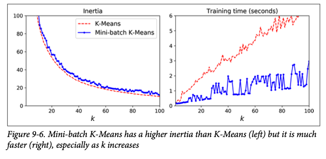
Even with all these speed-ups, if the data set is really large, then KMeans will be slow. For large data sets it is much better to perform KMeans on subsets of the data (minibatches) and then combine the results. This can be three to four times faster and can also handle a dataset that doesn't fit in memory. Of course, it will perform slightly worse, especially as K increases. It will also not have a strictly decreasing J.
from sklearn.cluster import MiniBatchKMeans
batchkmeans=MiniBatchKMeans(n_clusters=10)
batchkmeans.fit(X_train)
The full list of parameters:
MiniBatchKMeans(batch_size=100, compute_labels=True, init='k-means++',
                init_size=None, max_iter=100, max_no_improvement=10,
                n_clusters=10, n_init=3, random_state=None,
                reassignment_ratio=0.01, tol=0.0, verbose=0)
The main new parameter is to specify batch size.
Question 8.12.
When do we want a larger batch size and when do we want a smaller batch size? Answer
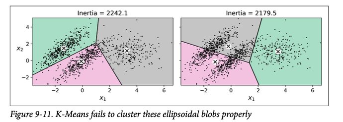
KMeans has many merits! Its fast and tends to work well on large data sets (especially with minibatch KMeans.) But the size, density and shape of clusters strongly impact KMeans. KMeans works best if clusters have similar size and density and a spherical shape.
There are other methods of clustering that will work better for some types of data, but KMeans works surprisingly well in a wide variety of cases. We will conclude with an example of color segmentation. For an image we will cluster colors to reduce the number of colors used in the image, possibly for compression or some type of image detection/analysis. It is surprising how few colors we need to fully represent the image!