Section 3 Linear Regression
Subsection 3.1 Introduction
Linear regression is a type of supervised learning. The goal is to predict a continuous output or \(y\) value. For example, suppose we want to predict house values from the following features:
| index | zip code | square feet | year built | home price |
| 1 | \(x_1^{(1)}\) | \(x_2^{(1)}\) | \(x_3^{(1)}\) | \(x_4^{(1)}\) |
| 2 | \(x_1^{(2)}\) | \(x_2^{(2)}\) | \(x_3^{(2)}\) | \(x_4^{(2)}\) |
| \(\vdots\) | ||||
| \(m\) | \(x_1^{(m)}\) | \(x_2^{(m)}\) | \(x_3^{(m)}\) | \(x_4^{(m)} \) |
Question 3.1.
Which of these are features? Which are labels?
Of course, we should first separate into training and testing data, before applying any machine learning algorithm.
Overall goal: Learn a function \(F\) such that for input \(\vec{x}=[x_1, x_2, x_3]\) and output \(y \) we have
For our example, the input is the zip code, square footage, and year built, and the output is the price of the house. What kind of function \(F\) do we want? In the case of linear regression we want a linear function \(F\text{.}\)
Example 3.2.
Suppose we are interested in studying the number of bugs in our code based on how fast we've been writing code. What data do we need and what data corresponds to features and what corresponds to labels?
Features = \(x\) = speed of typing
Labels = \(y\)= number of bugs
| speed | bugs |
| 1 | 3 |
| 2 | 5 |
| 3 | 7 |
Our goal is to predict the number of bugs for any speed. That is, we want to find a function \(F(x)\) where we input the speed and \(x\) so that \(F(x)=y\) where \(y\) is a prediction for the number of bugs. Since we are using linear regression we need \(F(x)\) to be linear, thus \(F(x)=\theta_0 +\theta_1 x\) and we can solve for \(\theta_0\) and \(\theta_1\text{.}\) In this case, our data points are exactly linear and we know how to find the equation of a line! \(\theta_1\) corresponds to the slope which is 2 and \(\theta_0\) corresponds to the \(y\) intercept which is 1. Thus, for this data \(F(x)=1+2x\) will exactly predict the speed for our training data. To make a prediction for new data points, we can just plug it into our function. to predict the number of bugs at a speed of \(x=1.5\text{,}\) we have \(F(x)=1+2(1.5)=4\text{.}\)
In general, the machine learning goal for linear regression is to learn the values for \(\theta_0\) and \(\theta_1\text{.}\)
In the previous example our data was exactly linear, but this won't generally happen in the real world! Also we will have much larger data sets!
In general our data, \(X\text{,}\) will have \(m\) data points and each data point will have \(f\) features, and a label \(y\text{.}\) We want to learn a function
Note that we denote this value with \(y^*\) because we will not generally get the exact \(y\) value. \(y^*\) is an approximation to \(y\text{.}\)
Question 3.3.
What do we learn in a machine learning algorithm? Answer
Subsection 3.2 The Cost function
How should we find a good line? We need the line to be close to the data. To specify this we will use a cost function. The cost function is a measure of how well our model fits the data. There are lots of choices for what the cost function could be, but we will use the following cost function:
This cost function is referred to as the mean squared error. The squared error refers to the \(\left[ h_\theta(x_1^{(i)},x_2^{(i)}, \cdots, x_f^{(i)}) - y^{(i)} \right]^2\) We want to square the error because we don't want positive and negative error to cancel out. The mean corresponds to dividing by \(m\text{,}\) the number of data points. In this case we divide by \(2m\) because it will make things nicer later when we take derivatives.
Question 3.4.
Do we want the cost to be big or small? If we start with all \(\theta_i=0\) will the cost be big or small?
In general, we want to minimize the cost. The machine learning algorithm is going to look for values of \(\theta_i\) that will decrease the cost.
Subsection 3.3 Matrix Form
It will be much more convenient for calculations to restate our objectives in matrix form. In general our data, \(X\text{,}\) will have \(m\) data points and each data point will have \(f\) features, and a label \(y\text{.}\) We can represent \(X\) as an \(m \times f+1\) matrix and \(y\) as an \(m \times 1\) matrix where
We want to learn \(f+1\) values for \(\theta_i\) so we can represent \(\Theta\) as an \(f+1 \times 1\) matrix
We can now consider our function \(F(X)\) as simply matrix multiplication.
The goal is to find \({\Theta}\) such that \({X}{\Theta}=y^* \approx y \text{.}\)
Perhaps the column of 1s in the \(X\) matrix is surprising. Note that this column is necessary in the matrix multiplication because of the bias term \(\theta_0\text{.}\)
We learn the \(f+1\) values for \(\theta_i\) by minimizing the cost function \(J\text{.}\) The mean squared error function in matrix form corresponds to
Example 3.5.
We return to examining the number of bugs in our code based on the speed of writing the code. We can rewrite \(X\) and \(y\) as
From \(X\) and \(y\) we learned
since
Note in this case we could solve for \(\Theta\) exactly with \(X\Theta=y\text{,}\) so that the cost function \(J=0\text{.}\) In general, we won't be have data that is so nice that we can solve for \(\Theta\) exactly. Instead, we will need to minimize the cost function \(J\text{.}\)
Subsection 3.4 Minimizing the cost function
How do we minimize a function? Answer
The idea is that we minimize \(J\) by setting all the partial derivatives equal to 0. We won't due the full derivation here, (see posted notes for details) but the point is that we can do it and solve the equations for \(\Theta\) and we get
This is called the normal equation.
Great news! We're done! This is exact and it works. And its fun to do Calculus!
Not so great news. This isn't an easy calculation to do. Finding an inverse for a large matrix is computationally expensive.
*** Add an example of large data set?? **Bad news. Sometimes the inverse doesn't exist because the matrix is not invertible!
Question: What should we do instead? Gradient descent. Coming next time!
Example 3.6.
We use the normal equation to solve for \(\Theta\) in our simple example of examining the number of bugs related to the speed of typing. Our data corresponds to
We want to solve for
Switch to Jupyter Notebook example here. https://colab.research.google.com/drive/1WwdRLc-x9W-C_sJ5Zt4dIb2JTHa7KHoI?usp=sharing
Subsection 3.5 Gradient Descent
***** Note: This section is not completely finished!!! *****
We will go through the the steps of gradient descent carefully in this section. We will not do this for every type of optimization, but the ideas are similar so we want to understand at least one.
Question 3.7.
Brief Review. We defined a lot of terms last time: \(X, y, h_\Theta(X), J,(X^T X)^{-1} X^T y\text{.}\) What do they all mean and what are they used for? Which ones are for training and which are for testing?
Answer\(X\) is a matrix where the columns are features and the first column is all ones. \(y\) is the labels. \(h_\Theta=X \Theta \) is model. We assume a linear model. \(J\) is the cost function which is the mean squared error. We minimize it to find \(\Theta\text{.}\) \((X^T X)^{-1} X^T y\) is the normal equation. It gives an exact answer for \(\Theta\text{.}\) The training stage uses a subset of \(X\) and \(y\) and involves creating the model, and minimizing the cost function to solve for \(\Theta\text{.}\) The testing stage involves making predictions on our test set. We hope \(y \approx X \Theta\text{.}\)
Today we will blow up the normal equation part. In real life we need approximate methods, because the normal equation will not work.
Question 3.8.
Why can't we use the normal equation? Answer
This is a simplified example that doesn't really correspond to machine learning yet. How do we find the minimum of the function \(y=2x^2+x+1 \text{?}\)
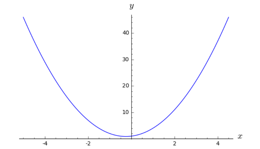
In this case, its easy to graph the function and at least approximate the minimum. But we want to talk about a strategy that will work when we can't easily see the minimum. For this iterative process, we will start with an initial guess. Maybe its a random guess, maybe its an educated guess, maybe we'll just pick \(x=1\text{.}\)
Question 3.9.
If we have a smooth function with only one minimum then, how do we use Calculus to find the minimum?
Step 1: Pick a starting value for \(x \) and check the derivative. We will pick \(x=1\text{,}\) \(y^\prime(1)=4\text{.}\) This value is not zero, so we are not at the minimum.
Step 2: Take a step in the right direction. How do we move closer to the minimum? The slope at \(x=1\) is positive so we want to move to the left. We want to move in the direction of the negative slope. Ok, so we should move left, but how far left should we move? This is a big question. We don't really know ahead of time. We will take a step that is proportional to the slope. \(step= \alpha*(slope)\text{.}\) The idea is that if the slope is large we are probably far from the minimum so we want to take a big step, but if the slope is small then we may be close to the minimum so we want to take a small step. \(\alpha\) is usually called the learning rate. The value of \(\alpha\) is something we have to choose, and depends on the data set. But generally we want to pick a small \(\alpha\text{,}\) say \(\alpha=.1\text{.}\)
We want to move from our current value of \(x=x_{old}\) by a step of \(\alpha*(slope)\text{.}\) Thus,
Repeat steps 1 and 2 until (hopefully), the value of the derivative is near zero. We can explore this in the Sage code below.
This is the idea of gradient descent! There are lots of more other optimization methods. But they generally follow this iterative or stepping style. BFGS, Newton-Conjugate-Gradient, ADAM are methods we'll see these in some of our later machine learning algorithms.
Question 3.10.
What happens if \(\alpha=.01\text{?}\) \(\alpha=.5\text{?}\) \(\alpha=1\text{?}\)
AnswerTry it and see!
\(\alpha\) is an optimization parameter. We choose it. This is often called a hyperparameter of the optimization method. Parameters of the model would be the \(\theta\) values. Hyperparameters are features of the optimization technique. They impact how quickly or how well we can find the theta values. Note that if \(\alpha\) is too small, it will take a long time to find the minimum. (We don't want our program to run for days/weeks/years...) If \(\alpha\) is too large, we can miss the minimum entirely and get larger and larger values for \(x\text{.}\) Eventually this will crash our program with NaNs. Finding the right balance between computation speed and accuracy is the goal here. For example, with \(\alpha=0.1\) we see that the answers are converging to \(x=-.25\) fairly quickly. Generally, \(\alpha\) is less than 1 and usually much smaller. We might start with \(\alpha=0.1\) or \(\alpha=0.01\) in large data sets. Note that we don't want to pick negative values for \(\alpha\) because then we will be moving away from the minimum rather than closer to it.
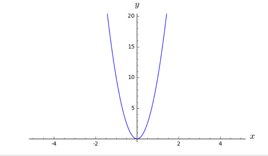
Hooray for gradient descent! But now we want to get back to our machine learning problem and do this in multiple dimensions! Remember the function that we are trying to minimize is
This function is convex (concave up) and smooth, so gradient descent will work well.
NOTE: Not all cost functions or optimization problems are this nice.
So what does gradient descent look like for linear regression? We are trying to solve for \(\Theta\) and we need to step in the direction of the negative derivative of \(J\text{.}\) We are in the multivariable case here, so we actually use partial derivatives, \(\frac{\partial J}{\partial \Theta_j}\text{.}\) Thus, we start with a initial value \(\Theta_j^{old}\text{,}\) and step to a new value
Restating this in matrix form gives
Important! Feature scaling (also called normalization) is very important! x
Subsection 3.6 Implementation
The sklearn code for implementing linear regression should feel familiar.
from sklearn.linear_model import LinearRegression
lm = LinearRegression()
lm.fit(X_train, y_train)
lm.predict(X_test)
lm.score(X_test,y_test)
As usual the .fit creates the model for linear regression and .predict applies the model. The attributes lm.intercept_ lm.coef_ give the intercept and slope for the linear model.
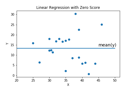
The attribute .score is a bit more complicated. It returns the coefficient of determination \(R^2\) of the prediction. The coefficient \(R^2\) is defined as \((1 - \frac{u}{v})\text{,}\) where \(u\) is the residual sum of squares
and \(v\) is the total sum of squares
where \(m=\operatorname{mean}(y_{true})\text{.}\) The best possible score is 1.0 (perfect fit!) and scores range from \((-\infty,1)\text{.}\)
When does the score =0? \((1 - \frac{u}{v})=0\) so \(u=v\) which means the model is always predicting the average value of \(y\text{.}\) But this is cheating, we could do this without any fancy machine learning algorithms. This is really underfitting our data and we want to know!
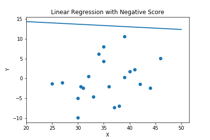
Question 3.11.
What model have we seen that always predicts the mean value of the data? AnswerIf the score is negative then the model doesn't match the data at all. For example score -7.3531279 in the image below. In this case, a linear model from one data set, was applied to a different data set. Our model is extraordinarily bad in this case.
To use LinearRegression function:
- Input \(X\) and \(y\)
- \(X\) is data, for \(f\) features and \(m\) data points, \(X\) should have shape\((m,f)\text{.}\) [Must be 2D array.] The LinearRegression function automatically adds the ones column to \(X\text{.}\)
- \(y\) is labels, can have shape \((m,)\) or shape \((m,1)\) but shape \((m,)\) will output a little nicer. [Can be 1D or 2D array. 1D is nicer. The shape of \(y\) effects the shape of the attributes
lm.intercept_lm.coef_.] - Either dataframe or numpy array is ok.
- It has four main parameters
LinearRegression(copy_X=True, fit_intercept=True, n_jobs=None, normalize=False)
Parameter Notes:
- The
copy_X=Truemakes a copy of the data before manipulating it. This is good practice in general, because you might overwrite your data. However, with a huge data set this may take a lot of memory. - The
fit_intercept=Trueallows the line to have a non-zero \(y\)-intercept. Thefit_intercept=Falseforces the line to go through the origin. This is an option for the type of model that you want. - The
n_jobs=Nonehas to do with parallelization of code which we are not going to need. (But in real life, you might!) - The
normalize=Falsemeans it does not do any automatic scaling of the data. Ifnormalize=Truethen it applies normalization. In this case normalize means subtracting the mean and dividing by the l2-norm \(=\sqrt{(x_1-m)^2+(x_2-m)^2+ \cdots + (x_k-m)^2}\) where \(m\) is the mean. This is not the same as StandardScaler which subtracts the mean and divides by the standard deviation/variance. Which should we use? Normalize or StandardScaler? AnswerWe will primarily stick to StandardScaler. But in real life it depends on data set and goals. Doesn't always matter. But use one!\begin{equation*} X=[1,2,3,4,5] \end{equation*}\begin{equation*} X.mean()=3. \end{equation*}\begin{equation*} X-X.mean()=[-2,-1,0,1,2] \end{equation*}\begin{equation*} X.std()=\sqrt{2} \end{equation*}\begin{equation*} StandardScaler(X)=\frac{1}{\sqrt{2}}[-2,-1,0,1,2] \end{equation*}\begin{equation*} =[-1.414, -0.707, 0 , 0.707, 1.414] \end{equation*}\begin{equation*} \sqrt{(-2)^2+(-1)^2+0^2+1^2+2^2}=\sqrt{10} \end{equation*}\begin{equation*} Normalized(X)=\frac{1}{\sqrt{10}}[-2,-1,0,1,2] \end{equation*}\begin{equation*} =[-0.632, -0.316, 0 , 0.316, 0.632] \end{equation*}Sometimes normalization means something different (for example, using the MinMaxScaler). - LinearRegression uses the Ordinary Least Squares solver from scipy, solving the normal equation, with pseudoinverses. The pseudoinverses are a big improvement for computational efficiency but it will not generally work well for large data sets!!!
But wait? Didn't you say we should never use the normal equation and should always use gradient descent/optimization methods? Answer
The method of gradient descent previously described is also called batch gradient descent. It means we apply gradient descent to the entire batch of the data set. If the data set is large this is generally too computationally expensive. There are two main modifications of gradient descent, stochastic gradient descent and mini-batch gradient descent. For stochastic gradient descent just pick one point randomly rather than use the entire matrix of feature values. This will speed up each step of the calculation substantially, but it may take a long time to converge to the minimum or it may never converge to the minimum. Mini-batch gradient descent is in between using a single point and using the full data set. Chose a small number of points instead of just one. The computations are more work than stochastic gradient descent, but still less work than the full data set. But it will probably be more accurate and converge faster since it is using more of the data set.
For these algorithms we may have additional hyperparameters. We could run through the data set multiple times, these are called epochs or we could change the learning rate over time, usually larger at first and then smaller.
The code in sklearn is
from sklearn.linear_model import SGDRegressor
sgd_reg = SGDRegressor()
The main attributes are the same as LinearRegression but there are many more hyperparameters!
SGDRegressor(alpha=0.0001, average=False, early_stopping=False, epsilon=0.1,
             eta0=0.01, fit_intercept=True, l1_ratio=0.15,
             learning_rate='invscaling', loss='squared_loss', max_iter=1000,
             n_iter_no_change=5, penalty='l2', power_t=0.25, random_state=None,
             shuffle=True, tol=0.001, validation_fraction=0.1, verbose=0,
             warm_start=False)
We've discussed a few of these parameters, eta0=0.01 is the learning rate and loss='squared_loss' refers to using means squared error as the cost function. fit_intercept=True is the same as in the LinearRegression case, and indicates whether or not to allow a \(y\)-intercept.
These parameters fall under the following categories:
-
Cost(=Loss) Function.
loss='squared_loss'refers to using mean squared error as the cost function.epsilon=0.1is a parameter of some of the other loss functions. -
Learning Rate and Schedule.
eta0=0.01is the learning rate. We've been calling this \(\alpha\text{.}\)learning_rate='invscaling'is the learning schedule.learning_rate='constant'always uses the same value for \(\alpha (=\eta)\text{.}\)power_t=0.25is a parameter of the learning schedule. -
Stopping and Starting Conditions.
tol=.001andn_iter_no_change=5are stopping conditions.warm_start=False(indicates whether or not to reuse the solution of the previous call to fit as initialization.) -
Epoch Conditions. The number of epochs refers to the number of passes over the training data. These parameters include
max_iter=1000shuffle=True(shuffles the data after each epoch), andaverage=Falseindicates whether or not to average SGC weights over multiple epochs forcoef_. -
Regularization Parameters. The regularizer is a penalty added to the loss function that shrinks model parameters towards the zero vector. We'll talk more about this later. These parameters include
alpha=0.0001, early_stopping=False, penalty='l2', l1_ratio=0.15. Note this \(\alpha\) is not the learning rate.
We will come back to some of these as we learn more techniques (especially regularization), but for now we are going to skip these details.
Learning Curves allow us to evaluate our choice of \(\alpha\text{.}\) For a specific \(\alpha\) value, keep track of \(J\) values as run through iterations. Then plot the cost as a function of the number of steps and analyze the graph. Is \(J\) decreasing? Did we take enough steps? Did we take too many steps? Is this a good choice of \(\alpha\text{?}\)
Switch to Jupyter notebook here.
https://colab.research.google.com/drive/157qmtWQ3HK6bxlwDjtbqkeVSSZYEYIqO?usp=sharing