
Section 5 Polynomial Regression
Subsection 5.1 Introduction
Suppose we want to apply regression or classification techniques to data sets as in Figure 5.1. 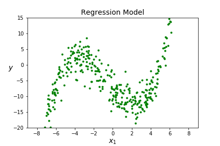

Question 5.2.
Will linear regression be a good choice for the regression data? Will logistic regression be a good choice for the classification data? Why or why not? Answer
Question 5.3.
Where should we make changes in our six step summary?Process Data for \(X\) and \(y\text{.}\)
Learn Function \(F\) such that \(F(X) \approx y \text{.}\)
Choose a Model.
Choose a Cost Function.
Solve for \(\Theta\text{.}\)
Make Predictions!
Example 5.4. One Feature.
Suppose we have one feature, \(x_1\text{.}\) Then our linear regression model would have
we could convert this to allowing a polynomial of degree 3 by
Note that \(F\) is not linear in \(x_1\text{,}\) but it is still linear in \(\Theta\text{.}\)
Question 5.5.
Why? Answer
to
Note that we are only adding polynomial terms to our features and not to our bias term, 1. A constant to any power is still a constant after all.
Hmmm. We increased from 2 to 4 \(\Theta\) parameters. What do we think about that?
Question 5.6.
How many \(\Theta\) parameters would there be if there is one feature and a degree 10 polynomial? One feature and a degree \(d\) polynomial? AnswerExample 5.7. Multiple Features.
Its more complicated with more features because we need to remember all the cross terms between features. For a data set with two features we want to change
into a polynomial of degree 3 by
Again, note that \(F\) is not linear in \(X_p\text{,}\) but it is still linear in \(\Theta\text{.}\) Thus, we can (and will!) think about polynomial regression as linear regression (or logistic regression) but on more features. So we will change
to
Hmmm. We increased from 3 to 10 \(\Theta\) parameters. What do we think about that?
Question 5.8.
How many \(\Theta\) parameters would there be if there are two features and a degree 4 polynomial? Answer
Question 5.9.
How many \(\Theta\) parameters are there if we have 3 features and use a degree 5 polynomial? What about \(f\) features and use a degree \(d\) polynomial? Answer
Question 5.10.
Where does that formula come from? Hint
Let's go back to our example of \(f=3\) and \(d=5\) and outline each of the cases for combinations of numbers and features. The set \(S= \{ 1,2,3,4,5,X_1,X_2,X_3 \} \text{.}\) We need to choose three objects and from those three objects construct an \(X_1^aX_2^bX_3^c\) where \(a+b+c \leq 5\)
We thus see that the number of \(\Theta\) parameters should indeed correspond to
Subsection 5.2 Implementation
In the previous section we saw that the idea for implementing polynomial regression is to
- Add polynomial features to our data X
- Perform Linear Regression (or Logistic Regression) on the enhanced data set X.
We already know how to implement Linear and Logistic Regression, so we just need to know how to add polynomial features to our data. We will implement this with the PolynomialFeatures() tool from sklearn.
from sklearn.preprocessing import PolynomialFeatures
poly_features = PolynomialFeatures(degree=3, include_bias=False)
X_poly = poly_features.fit_transform(X)
In this case, \(X\) is our original data set, degree=3 specifies the degree of the polynomial model, and include_bias=True will add the column of ones, include_bias=False does not. (Usually we do not need to add the column of ones because the ML algorithms in sklearn will do this for us.)
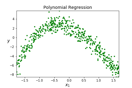
Let's return to one of the data sets from the introduction.
Question 5.11.
How many features in this dataset? AnswerQuestion 5.12.
Is this discrete or continuous data? AnswerQuestion 5.13.
What type of ML algorithm should we use? AnswerPolynomialFeatures() and LinearRegression().
Question 5.14.
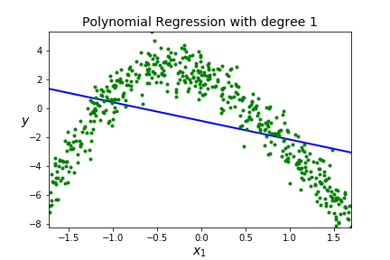
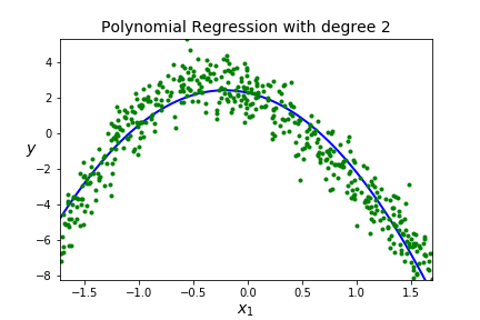
How does it look? What important steps did we skip? Answer
Question 5.15.
How important is scaling the data in polynomial regression? Answer
We now have multiple preprocessing steps that we need to apply to transform our data, first on training data and then on testing data. It can get complicated with so many steps, so we are going to use a tool from sklearn called Pipeline. Pipeline allows us to sequentially compose a list of transformations and conclude with an estimator. For us the transformations will be the data processing steps and the estimator will be the machine learning algorithm. Pipeline will call .fit_tranform on the list of transformations in the order they are listed, and will call .fit on the last estimator. The main parameter for Pipeline(steps, memory=None, verbose=False) is steps which is a list of (name,transform) tuples. To apply the steps
- Add polynomial features to data set
- Apply linear regression
we would create a pipeline with
from sklearn.pipeline import Pipeline
poly_model  = Pipeline([
    ('poly_feat', PolynomialFeatures(degree=3, include_bias=False)),
    ('lin_reg', LinearRegression()),
    ])
We interact with poly_model in the same way we would interact with LinearRegression(), or whatever the last item in our steps is. That is, we can create the model with poly_model.fit(X,y), apply the model with poly_model.predict(X) and score the model with poly_model.score(X,y).
Question 5.16.
What will poly_model.fit(X,y) do? What will poly_model.predict(X) do? What will poly_model.score(X,y) do? Answer
poly_model.fit(X,y) first calls PolynomialFeatures.fit_transform(X) and then calls LinearRegression.fit(X,y). So that it both creates the polynomial features and applies linear regression to the polynomial features to model the data.poly_model.predict(X) first calls PolynomialFeatures.fit_transform(X) and then calls LinearRegression.predict(X).poly_model.predict(X) first calls PolynomialFeatures.fit_transform(X) and then calls LinearRegression.score(X).
We can still access of the individual steps if we want, but it takes a bit more work. We method uses the named_steps attribute of the Pipeline. For example, poly_model.named_steps.lin_reg.intercept_ will give the intercept from the Linear Regression model. We can also access this by with poly_model['lin_reg'].intercept_.
Let's repeat our previous code using a Pipeline! Not we still haven't split into training and testing data yet, or applied feature scaling.
Question 5.17.
What doesintercept [-7.5258753] and coefficients [[-3.76629704 0.30092201 0.15046627]]. tell us about \(\Theta\text{?}\) AnswerIn general, the process we want for a real data set would be
- Take a look at the data and make sure you understand it.
- SPLIT the data (both features and labels) into Training and Testing Sets. (Eventually swap steps 1 and 2.)
- ADD relevant features to data set. (For example, add polynomial features).
- SCALE the FEATURES of the TRAINING data (fit_transform).
- TRAIN the model (fit) using the TRAINING data. (For example, apply linear regression.)
- TEST the model using the TESTING data.
- Experiment - How did your model do? Can you do better?
The last step is really important. Experimenting with the model is always part of your job as a data scientist!
Question 5.18.
For polynomial regression, which of these steps should be combined into a Pipeline and how would we do it? Answer
from sklearn.pipeline import Pipeline
poly_model  = Pipeline([
    ('poly_feat', PolynomialFeatures(degree=3, include_bias=False)),
    ('std_scaler', StandardScaler()),
    ('lin_reg', LinearRegression()),
    ])
Question 5.19.
Why is splitting the data not included in the Pipeline? Answer
Subsection 5.3 Underfitting and Overfitting
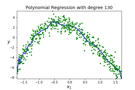
Suppose we have the following data set
| degree | score |
| 1 | 0.1566 |
| 2 | 0.8887 |
| 3 | 0.9217 |
| 4 | 4:0.9220 |
| 20 | 20: 0.9246 |
| 100 | 0.9254 |
| 125 | 0.9255 |
| 130 | 0.9200 |
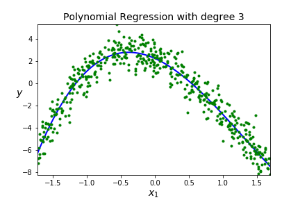
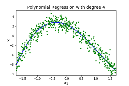

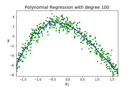
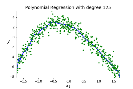
A BIG IDEA - You want to get a model that fits your data well AND generalizes well to new data sets.
Underfitting A model is underfitting if it is not matching the shape of the data, you assumed the wrong shape for \(F(x)\text{,}\) aka wrong model. High error when on the training data so the model just doesn't work, it won't be usefull on new data so high error on the testing data. You can see this by poor scores on both the training and testing data.
Overfitting A model is overfitting if it is matching the shape of the training data really well (too well!) It may go through a lot of points on the training data and will have low error on the training data. BUT, you have effectively memorized your data, so this model will not generalize well to new data so high error on the testing data. Scores are good on training data, but poor on testing data.
One way to visualize underfitting versus overfitting is to Plot Learning Curves. We will examine the score on the model as we increase the percentage of training data. Note this is a different use of the term Learning Curves than the Learning Curves from Gradient Descent. There "training" means how many steps of gradient descent we took. We were testing the optimization not the model. Now, we don't want to test how well the optimization is working. Rather, we want to know how our model reacts as it is given more training data.
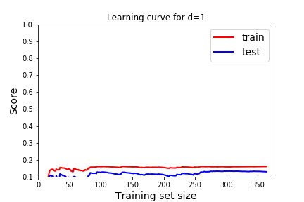
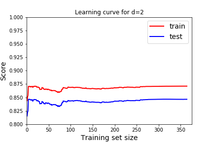
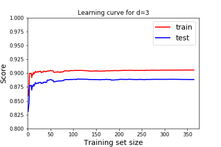
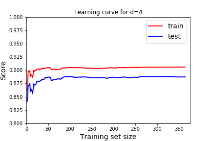
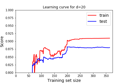
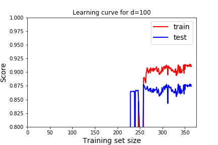
What should a learning curve look like for a good model? In all of these, we see that as we train with more data the model gets better at predicting the training data (red), but eventually reaches a plateau.
- We want the scores to be good on both training and testing. Remember good depends on the score we use. In this case, the R^2 score, 1 indicates a perfect fit, so we want the scores to be close to 1. For the cost function, or mean squared error we would want the scores to be close to 0.
- We expect the score to be better for the training data than the testing data. But we would like the score on the testing data to be close to the training data.
Question 5.20.
Which learning curve indicate underfitting and which learning curve indicates overfitting? How would we use these to pick the best degree of the polynomial? How does that usually correspond to degree of the polynomial? Answer
Jupyter notebook for implementation details of this type of learning curves and an example of using polynomial regression with logistic regression.
There are methods for searching the parameter space to find the best polynomial degree. See the next chapter. For now, experiment and get a feel for what these parameters do so that when you use the search features you understand what they are doing. There are also different measures of how well the model is doing. Start with a model, choose a small set of features, question every assumption that you made in your model test each assumption to see if you can approve take good notes for parameters