Section 7 Support Vector Machines
Are we ready for another machine learning algorithm? How about some Calculus?
Question 7.1.
What machine learning algorithms do we have so far? What are the main steps in most of our supervised machine learning algorithms?
Answer 1So far we have one unsupervised learning algorithms, Principal Component Analysis, and five supervised learning algorithms:
- Linear Regression
- Linear Regression with Polynomial Features
- Logistic Regression
- Logistic Regression with Polynomial Features
- k Nearest Neighbors
We generally have six steps in our regression models.
Get, process, clean data for \(X\) and \(y\text{.}\) Split into training and testing. Then explore/analyze training data set to understand the data. If necessary, perform feature scaling (fit on only training data, but applied to all data.)
Question 7.2.
Why should we perform data analysis on only the training data and not the testing data set? AnswerWe need the testing set to be an unbiased measure of the performance of our model. If we explore the testing set as part of our data analysis we are leaking information about the testing set to us (and therefore our model.) We've been blurring this line a bit because of the small size of some of our data sets, but as we move to larger data sets we want to be more careful about this. (And its very important for real world implementation.)Question 7.3.
When is feature scaling necessary? Why is it important? AnswerAlmost always. Its especially important if the data features have widely different scales. In most cases it impacts the convergence of the optimization technique. In some cases it also affects the ability of the model to make accurate predictions.Question 7.4.
Our parameter searching from last time actually adds a step here. What did we add? AnswerSplit data into train, validate, and test. Validation data is used to tune parameters/hyperparameters and testing is reserved for an unbiased estimate of final model that can be applied to data that was not used to build the model or tune the parameters.-
Learn Function \(F\) such that \(F(X) \approx y \text{.}\)
Question 7.5.
Which of our previous models do not learn a function that approximates \(y\text{?}\)
AnswerPCA is unsupervised so there is no y to approximate.
kNN does not learn a function, or follow this six step process. kNN memorizes the data and must search through the entire data set to find the \(k\) nearest points. It then makes a prediction based on majority vote.
-
Choose a Model.
Question 7.6.
What types of models have we used so far?
AnswerLinear, logistic and polynomial!
For the linear model
\begin{equation*} h_\Theta (X) = X \Theta . \end{equation*}For the logistic model
\begin{equation*} h_\Theta(X)=g({X}{\Theta})= \frac{1}{1+e^{-{X}{\Theta}}}. \end{equation*}(Also softmax model for multinomial logistic regression.)
Our polynomial model doesn't actually change the model, it just adds polynomial features.
-
Choose a Cost Function.
Question 7.7.
What did we recently add to our cost functions and what type of cost functions do we have so far? What are we looking for in a cost function in general?
AnswerWe added regularization here!
We are using either mean squared error in Linear Regression or log-loss (or cross entropy loss) in Logistic Regression (multinomial), plus an appropriate regularization.
For the mean squared error
\begin{equation*} J = \frac{1}{2m} \sum_{i=1}^m \left[ h_\theta(X^{(i)} - y^{(i)} \right]^2 + \alpha \sum_i \theta_i^2 \end{equation*}For log-loss
\begin{equation*} J= -\frac{1}{m} \sum_{i=1} ^m y_i\log(h_\Theta(X^{(i)})) +(1-y_i)\log(1-h_\Theta(X{(i)})) + \frac{1}{C} \sum_i \theta_i^2. \end{equation*}Note: this is ridge or l2 penalty regularization.
The important features of our cost function are some way to measure error in our prediction and a smooth/convex function that is easy to optimize.
Solve for \(\Theta\text{.}\)
Make Predictions!
Question 7.8.
What other fun and exciting topics are left in this class? AnswerSubsection 7.1 Introduction
Our next type of machine learning algorithm is called Support Vector Machines. Support Vector Machines (SVM) is one of the most popular and powerful machine learning algorithms. The idea was originally developed at AT&T Bell Laboratories The SVM algorithm dates to 1963 and work done by Vapnik and Chervonenkis. In the 1990's, Vapnik, Boser and Guyon expanded the model to include a non-linear component (kernel trick), and Cortes and Vapnik developed a more robust model for outliers (soft margin versus hard margin classification). It is based on statistical learning frameworks or VC theory and can be used for classification and regression. It can also be used for outlier detection, however it is especially powerful for classification of complex small to medium size data sets (up to approximately 50,000 data points). The idea is that we want a large margin classifier. What does large margin mean?
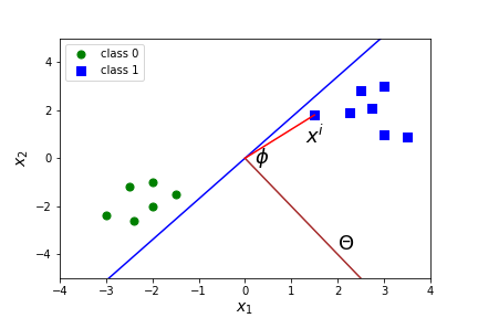
We will illustrate with the simple classification example below. In this case we want to find a linear decision boundary to separate the data set into two classes. Four lines are given that all separate the two classes of data.
Question 7.9.
Which decision boundary do we like the best and why? 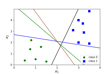
The idea for using support vector machines for classification is that we want to find a line that has the largest possible distance from all the points in the data set. There should be a large margin \(m\) between the line and the data, and a margin of \(2m\) between the two different data sets.

The points on the edge of the margin (points A and B) support the model. That is, adding more points would not change the decision boundary as long as they are outside the margin. These points are called support vectors.
The idea for using support vector machines for regression is similar except that we want the wide margin to contain all the points in our data set rather than separate them. 
Question 7.13.
Which aspects of our six step machine learning summary will we need to change? Answer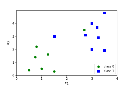

Subsection 7.2 Revising the cost function.
How we are going to revise the cost function and why is going to take some work! The idea is to use a modified version of the cost function for logistic regression. Recall that binary classification with logistic regression uses the log-loss cost function.
Note I've moved the minus signs back inside the sum here. There are three modifications that we will make to this function; two of them are minor notational changes and the last one is the substantial change.
-
Change \(\alpha\) to \(C\) and move from regularization term to cost term.
\begin{equation*} J= C\frac{1}{m} \sum_{i=1} ^m -y_i\log\left( \frac{1}{1+e^{-{X}{\Theta}}} \right) -(1-y_i)\log\left( 1-\frac{1}{1+e^{-{X}{\Theta}}} \right) + \sum_i \theta_i^2. \end{equation*}This is the same as replacing \(\alpha\) with \(\frac{1}{C}\) and multiplying by \(C\text{.}\) This is mostly a notational preference but it also indicates a shift in importance of the \(\sum_i \theta_i^2\) term. Note that now large values of \(C\) mean little regularization and low values of \(C\) mean lots of regularization.
-
Eliminate the constant \(\frac{1}{m}\text{.}\)
\begin{equation*} J= C \sum_{i=1} ^m -y_i\log\left( \frac{1}{1+e^{-{X}{\Theta}}} \right) -(1-y_i)\log\left( 1-\frac{1}{1+e^{-{X}{\Theta}}} \right) + \sum_i \theta_i^2. \end{equation*}This is also a minor change. We could view it as a minor notational change to replace the constant \(\frac{C}{m}\) with a different constant \(C\text{.}\) The important point is that \(\frac{1}{m} \operatorname{Cost}(\Theta)\) will be minimized at exactly the same place as \(\operatorname{Cost}(\Theta)\) so that eliminating the \(\frac{1}{m}\) will have no impact on the value of \(\Theta\) that minimizes the cost.
Question 7.15.
What value of \(x\) minimizes \(y=3x^2-12x\text{?}\) What value of \(x\) minimizes \(y=\frac{1}{3}(3x^2-12x)=x^2-4x\text{.}\) AnswerYay Calculus! We find the minimum by setting the derivative equal to 0! \(y'=6x-12=0\) if \(x=2\text{.}\) Similarly \(y'=2x-4=0\) if \(x=2\text{.}\)Question 7.16.
Can we just eliminate \(C\) also for the same reason? AnswerNo! The constant \(C\) controls the weighting between regularization and the cost function so eliminating \(C\) would result in a loss of flexibility in our model. Different values of \(C\) will change the value of \(\Theta\) that minimizes the cost.Question 7.17.
How? What does regularization do again? AnswerRegularization tries to control overfitting by constraining the size of \(\Theta\text{.}\) -
This is the big change!! Flatten the cost function into a piecewise linear function. Remember that we have two cases in the cost function, corresponding to the two classes of \(X^i\text{.}\)
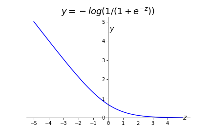
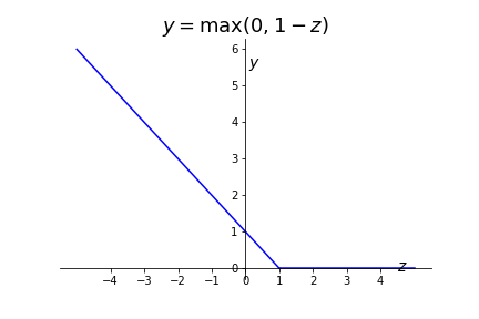
Figure 7.18. Cost Function if \(y^i=1\) (class 1) 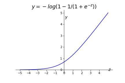

Figure 7.19. Cost Function if \(y^i=0\) (class 0) To convert this to a formula we first replace the log pieces with the piecewise linear pieces.
\begin{equation*} J= C \sum_{i=1} ^m -y_i\log\left( \frac{1}{1+e^{-{X}{\Theta}}} \right) -(1-y_i)\log\left( 1-\frac{1}{1+e^{-{X}{\Theta}}} \right) + \sum_i \theta_i^2\\ = C \sum_{i=1} ^m y^i \left(\max(0,1-X\Theta) \right) +(1-y^i)\left(\max(0, 1+X\Theta \right) + \sum_i \theta_i^2 \end{equation*}Then we have some fun with algebra! Remember that the \(y^i \) and \(1- y^i \) are either zero or one, so we are really just adding either \(\max(0,1-X\Theta) \) or \(\max(0,1+X\Theta).\) The only difference between these two pieces is the plus/minus sign. So we can combine this into a single piece with a new variable \(t^i\) to account for the plus/minus sign.
\begin{equation*} J = C \sum_{i=1} ^m \left(\max(0,1- t^i X \Theta) \right) \text{ where } t^i= \begin{cases} +1 \amp \text{ if } y^i=1 \\ -1 \amp \text{ if } y^i=0 \end{cases} \; \; + \sum_i \theta_i^2 \end{equation*}Question 7.20.
Do we need the new variable \(t^i\text{?}\) Could we specify this in terms of \(y^i\text{?}\) AnswerWe could definitely specify this in terms of \(y^i\) instead. Let \(t^i=(-1)^{y^i+1}\text{.}\) Yay, math!
Okay, we have a new cost function! This cost function is commonly referred to the hinge loss cost function. But why did we do this?!?
Question 7.21.
What aspect of the function \(\max(0,1\pm X\Theta)\)
Question 7.22.
What was the goal of support vector machines again? Answer
Question 7.23.
When is \(\max(0,1\pm X\Theta)\) equal to zero? What is \(J\) in that case? Answer
Question 7.25.
What does \(\|\Theta\| \) notation mean? Answer
Question 7.26.
Suppose \(\Theta=(0,\frac{1}{2},1)\text{.}\) What does \(X \Theta=0 \text{,}\) \(X \Theta=1 \text{,}\) \(X \Theta=-1 \) correspond to? How many features are there? Answer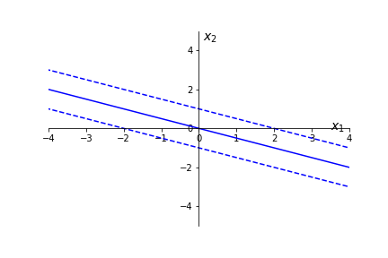
Question 7.27.
Why will the black line have a lower cost than the blue line? 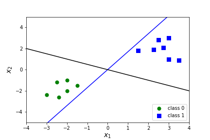
Question 7.28.
When is a dot product equal to zero? Answer
Question 7.29.
What is \(X \cdot \Theta\) in general? That is, what is the formula for a dot product? Answer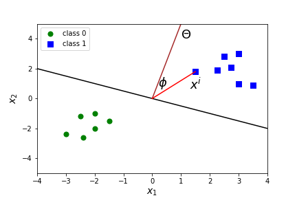
In summary, the cost function
The first term in this function essentially computes the sum of the margin violations. It will be zero if the point is outside the margin and on the correct side of the margin for its class. If it is not zero it will be related to the distance to the decision boundary. Minimizing this term ensures that the model makes the margin violations as small and as few as possible.
The second term will push the model to have a small weight vector \(\Theta\) which corresponds to a larger margin.
Question 7.30.
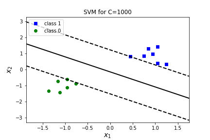
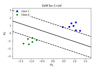
What is the value of \(C\) doing in our model? The value of \(C\) must be positive. What happens in the extreme cases? What happens if \(C=0\text{?}\) What happens if \(C=\infty\text{?}\)
AnswerIf \(C=\infty\) then we only care about the first term and do not care about the second term. That is, we do not care about a large margin, we only care about margin violations. This will produce a hard margin model. All points must be outside the margin. You can try this value in the model, with C=float("inf").
If \(C=0\) then we only care about the second term and do not care about the first term. That is, we do not care about margin violations, we only care about a wide margin. This will produce a soft margin model. Note that \(C=0\) is not positive and this is not actually a valid parameter for the model.
Of course, we don't usually want to be at either of these extremes and the goal is to find the right balance between the hard margin and the soft margin.
Subsection 7.3 Linear Implementation
The are several ways to implement SVM for classification with linear models. The most efficient is usually from sklearn.svm import LinearSVC and would be implemented as LinearSVC(C=1000, loss="hinge", random_state=42). We will specify the loss="hinge" to correspond to the cost function discussed above. The default loss is squared_hinge which, not surprisingly, squares the hinge loss. The disadvantage of this is that the linear function becomes a quadratic function, but the advantage is that there is no longer a non-differentiable point. This model will punish large errors more significantly than small errors, which may or may not be helpful. We will stick with the hinge loss, but in general you should consider which loss is most beneficial for your situation.
Question 7.31.
What does C=1000 mean in the model? AnswerC will mean little regularization. This is an important parameter to tune in our model.
  LinearSVC(penalty='l2',loss='squared_hinge',dual=True,
    tol=0.0001,C=1.0,multi_class='ovr',fit_intercept=True,
    intercept_scaling=1,class_weight=None,verbose=0,
    random_state=None,max_iter=1000)
Most of these parameters should look familiar by now. We can use the attributes .intercept_ and .coef_ to find the equation of the decision boundary and calculate the margin. As usual we can use .predict to make predictions on new data.
Question 7.32.
What is the margin? How do we calculate it from .intercept_ and .coef_? Answer
Let's look at applying SVM to our simple data set from before. It's too small to train/test split, but feature scaling is incredibly important to SVM so we will create a Pipeline to combine StandardScaler and LinearSVC.
Let's graph our decision boundary and margins! Remember that our decision boundary is \(X \Theta=0 \) which corresponds to
and the margins are just shifts of this by \(\frac{1}{\theta_2}\text{.}\)
Question 7.33.
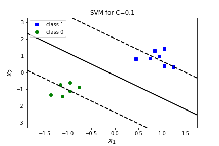
What happens if we change the value ofC=float("inf")? What about C=.1? C=.001? Answer| C=1000 | C=inf | C=0.1 | C=0.001 | |
| \(\theta_0\) | 0.108 | 0.108 | 0.080 | 0.001 |
| \(\theta_1\) | 0.685 | 0.685 | 0.611 | 0.013 |
| \(\theta_2\) | 0.730 | 0.730 | 0.454 | 0.012 |
| margin | 1.369 | 1.369 | 2.204 | 82.189 |

Subsection 7.4 Kernel Trick
In many cases a line is too simple to separate data points effectively. In this case, we can add more features, which is referred to as a kernel. The first type of kernel is a polynomial kernel. For a polynomial kernel we add polynomial features to our data set. (Just like we did for polynomial regression!) We can then find a linear separation in a higher dimensional space.
Example 7.34.
An example of a one dimensional data set is given on the left. There is no way to separate this data with a line! In the image on the right we have added a second feature \(x_2=(x_1)^2 \) and expanded to a second dimension. We can now separate the data with a line! 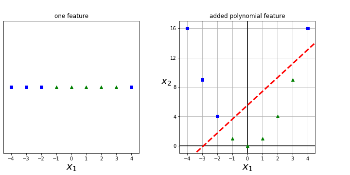
The kernel trick refers to a technique to make use of all the additional polynomial features without actually having to explicitly construct them. We could do this by using the PolynomialFeatures() and adding it to our Pipeline, but there's an even easier way, using SVC instead of LinearSVC.
We implement SVC with a polynomial feature by using kernel ="poly" and we will need to explore the best choice of parameters degree, C, and coef0. The hyperparameter coef0 controls how much the model is influenced by high- degree terms versus low-degree terms. Small values of coef0 will be closer to a linear decision boundary (favor the low degree terms) and and high values of coef0 will emphasize the high degree terms.
The coef_ attribute is not valid any more for a non-linear kernel, but there is a new attribute that allows us to examine the support vectors support_vectors_ .
.predict. Question 7.35.
What do you think happens as we varyC? AnswerBut maybe polynomial features aren't really what we want. Another way to add features is to create new features that measure the similarity of each data point to a set of landmarks. This kernel is called the Radial Basis Kernel and uses the Gaussian Radial Basis function to determine similarity. Let \(l \) be a landmark point then the Guassian Radial Basis function is
Remember that \(\| x-l \|\) is the Euclidean distance from \(x\) to \(l\text{.}\)
Question 7.36.
Consider the landmark \(l=0\text{.}\) What does \(e^{-\gamma x^2 }\) look like? What is \(\gamma \text{?}\) What does adding this add a feature tell us about our data? Answer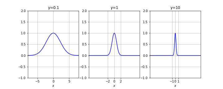
Question 7.37.
What happens as we vary \(\gamma\) and \(l\text{?}\) Answer
Thus, the idea here is to use each landmark to create a feature.
Question 7.38.
What should we use for landmarks? Answer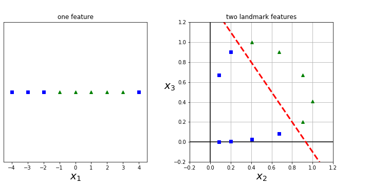
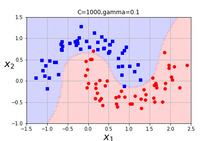
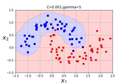
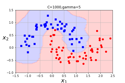
We implement this similarly with SVC using kernel ="rbf" and we will need to explore the best choice of parameters gamma and C.
Question 7.39.
What is the impact of varying gamma and C? When will C overfit? When will gamma overfit? How do we vary between hard margin and soft margin classification? Which of these combinations seems the best? 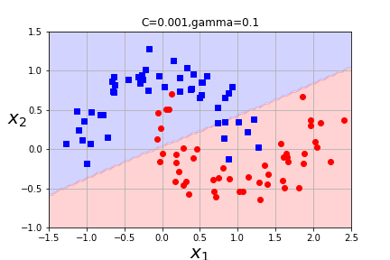
Other kernels are possible, but there are some conditions that must be satisfied in order to apply the kernel trick. (See your text for details about Mercer's Theorem if you are interested. Chapter 5, p. 171.) Generally, Radial Basis Kernel is most frequently used kernel with SVC(and is the default kernel.) You can also use SVC with a kernel=linear, but LinearSVC uses a different optimization strategy (liblinear versus libsvm) and will work better for larger data sets.
Question 7.40.
That's a lot of kernels! How do we decide which to use? Answer
Question 7.41.
What is the dual parameter in SVC? Answer
Question 7.42.
There are a lot of hyperparameters to tune. How do we do that? Answer
- Feature scaling is very important to the models performance (and not just for the optimization)! Some features may be ignored without feature scaling.
- In order to apply the kernel trick, there is also a slight modification to the regularization part of the cost function. The \(\sum \theta_i \) is replaced with \(\Theta^T M \Theta \) where \(M\) depends on the kernel and is chosen for computation reasons. Note that if \(M\) is the identity matrix, then it is almost \(\sum \theta_i \text{.}\) Why almost? Answer\(\theta_0\) is included in \(\Theta \) but not \(\sum \theta_{i=1} \text{.}\)
- For support vector machines, the output of a model when predicting on a new data point is a class rather than a prediction. (This is different from logistic regression. )
- There's a lot more cool stuff to know about support vector machines!! Check out Chapter 5 of Hands-on Machine Learning