Section 9 Neural Networks
Neural networks are some of the newest and most exciting machine learning models. However, neural networks build off the ideas that you have learned so far. Neural Networks may also be called artificial neural networks (ANN) or deep learning. The goal is to create a machine learning algorithm that can handle really complex problems. Neural networks are already used in a wide array of applications!
- image classification
- speech recognition
- recommendations (video and others)
- fake videos, or photos, or text, or ... (GANs = Generative Adversarial Networks)
- writing text
Subsection 9.1 Artificial Neurons
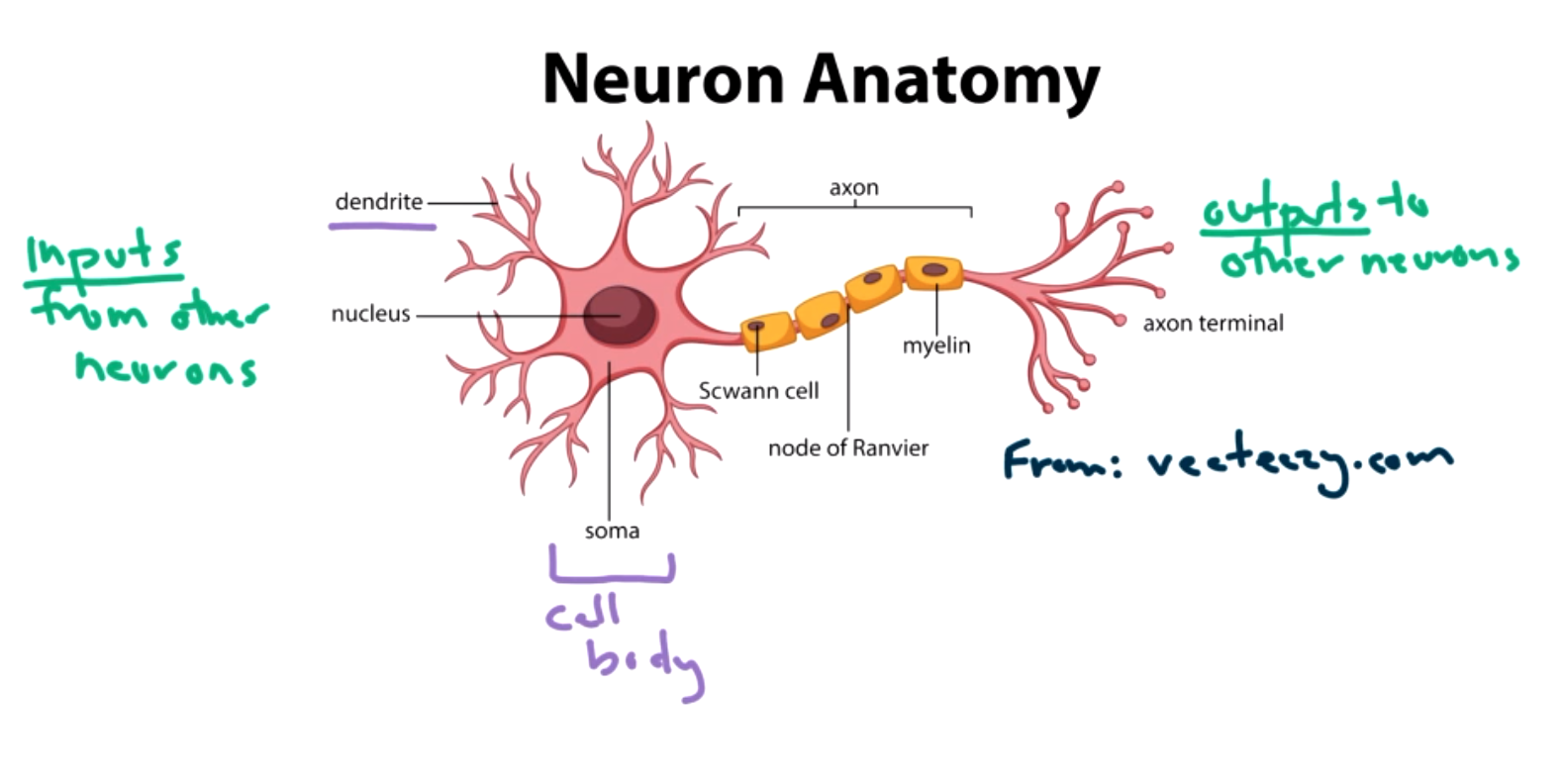
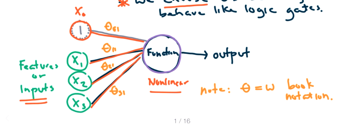
We will begin with an intuitive approach. Neural networks are modeled based on how the human brain works.
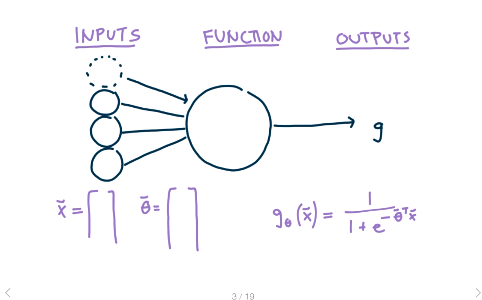
The activation function determines how strongly the neuron should react to the input, or if it should react at all. There are many different choices for the activation function, for example the hinge loss function or a linear function. However, linear functions end up being too simple, so we generally want some non-linear activation function. The output \(g\) represents the output of the activation function. In the simplest case, this will be the answer to our question of making a prediction for the input \(X\text{.}\) The first addition we are going to add to this model is to add weights to each of the inputs.
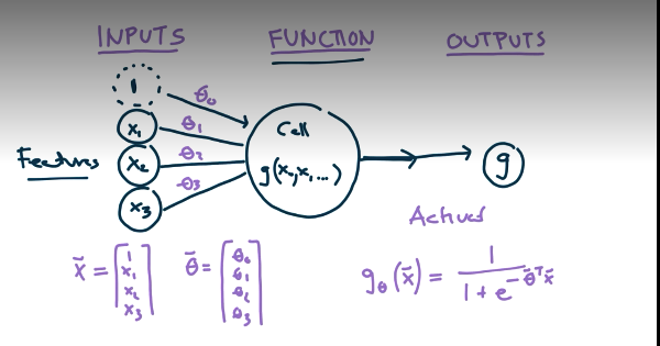
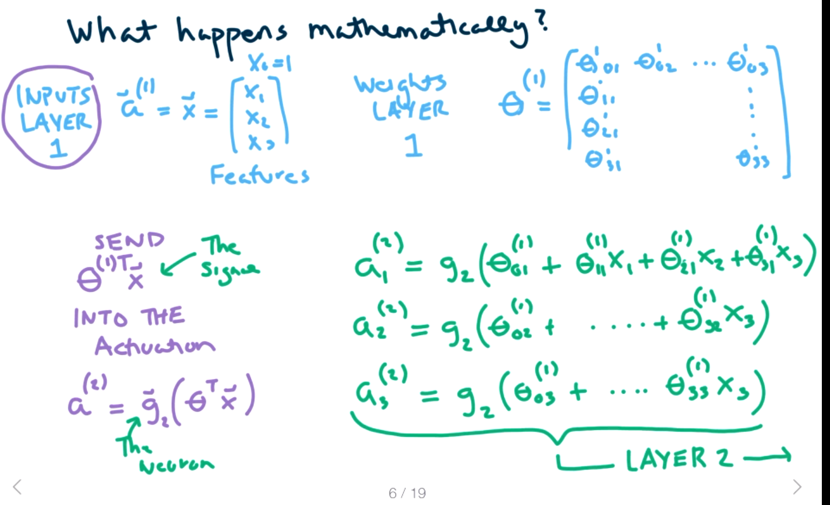
The new process is that the input features are multiplied by the \(\Theta\) values and then activated with a sigmoid function.
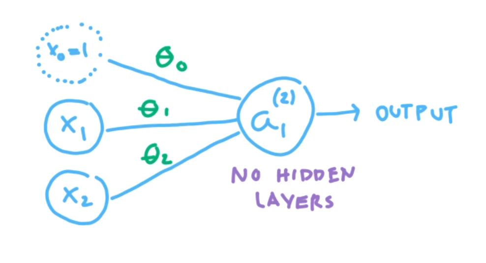
Question 9.1.
This should feel really familiar? If there is just a single neuron what process are we implementing? Answer
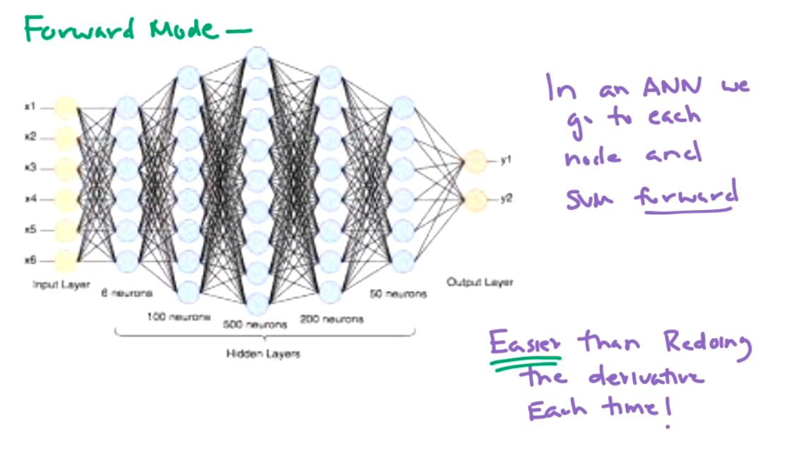
So how do we turn a single neuron into a neural network? Add lots of them and multiple layers of neurons!
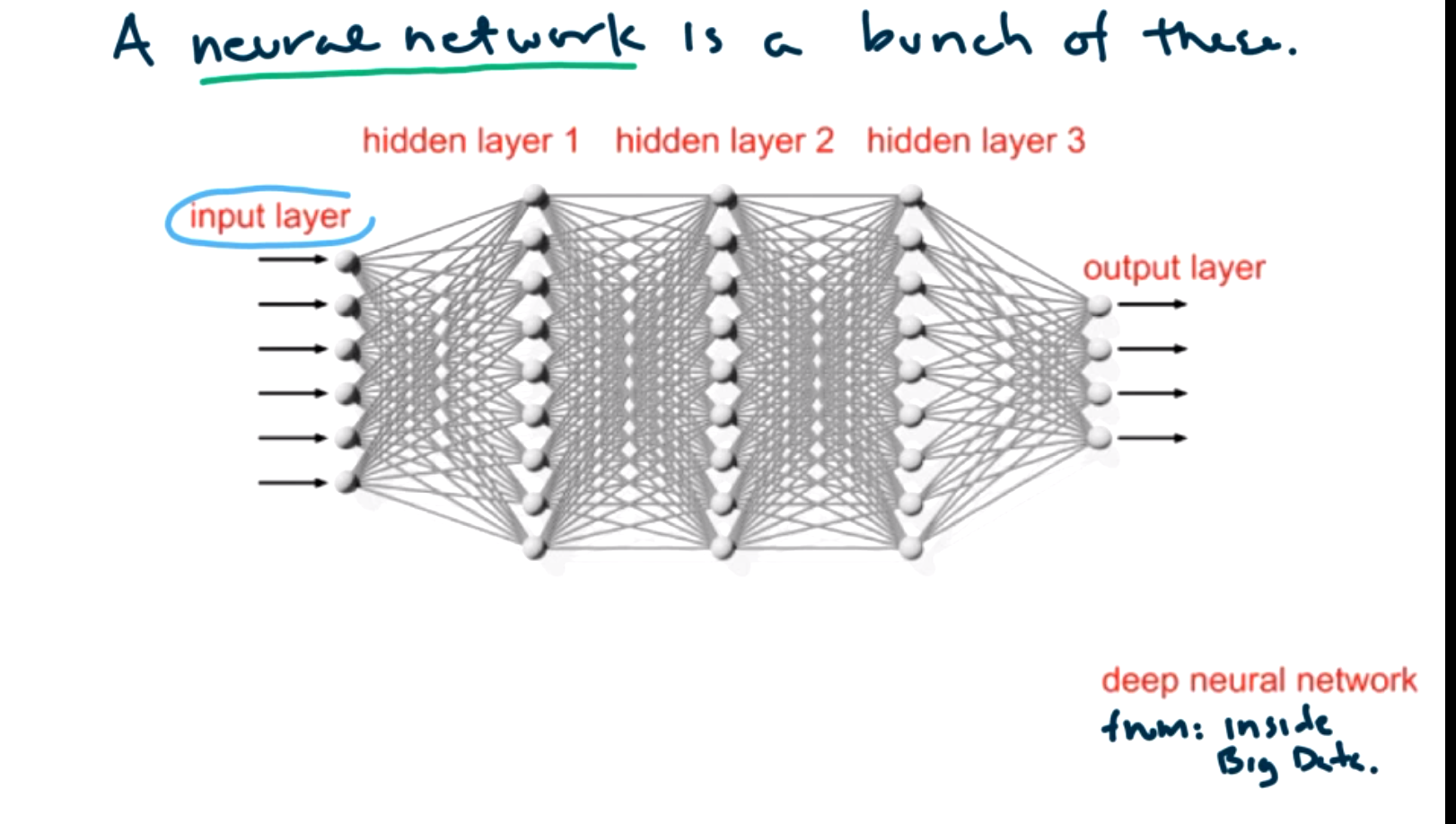
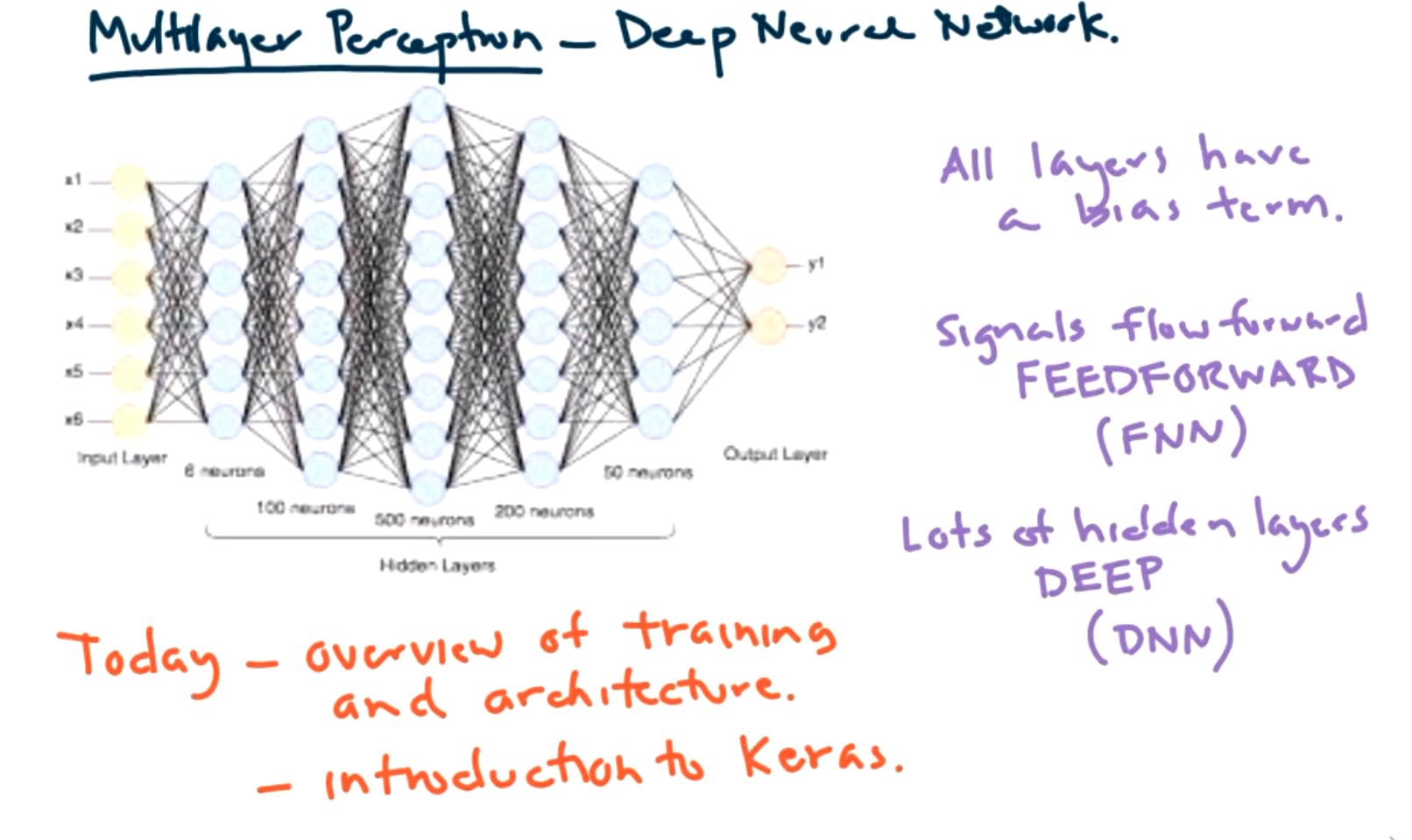
The input layer still corresponds to the features. (The bias term is still here, but it is not generally included in neural network diagrams.) In this image, there are three hidden layers, but there could be any number of these hidden layers in general. They are called hidden because the inputs and outputs of these layers are hidden inside the model. The depth refers to the number of hidden layers. The width refers to the number of neurons per layer. Each layer can have a different number of neurons. The output layer is always the last layer and corresponds “the answer”, that is, the prediction for input \(X\) based on our model. At each layer, the outputs from the previous layer are the inputs for the next layer. The \(\Theta\) values correspond to the weights on each of the lines between layers.

We will introduce some notation using a simpler example.
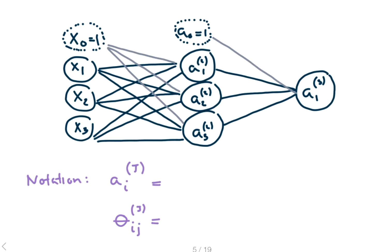
\(\theta_{ij} ^{(J)}\) maps from unit \(i\) in layer \(J\) to unit \(j\) in layer \(J+1\text{.}\)
\(a_i ^{(J)}\) represents the activation of unit \(i\) in layer \(J\text{.}\)
In this example, there are three input features in the input layer, three activation units in the hidden second layer, and a final output in the third layer. The output in the third layer is the answer or prediction for \(X\text{.}\) There will be two sets of \(\Theta\) values in this example, one from layer 1 to layer 2, \(\Theta_{12}\text{,}\) and one from layer 2 to layer 3, \(\Theta_{23}\text{.}\)
Question 9.2.
What dimensions will the \(\Theta_{12}\) matrix have? What about \(\Theta_{23}\)Answer
When building a neural net, we need to
- Choose the architecture (choose depth and width and activation, choose features, scale features, etc.)
- Train the neural network (solve for theta values, use an optimizer, but more later. vary learning rates, and regularization.)
- Tune and test (hyperparameter tuning, depth, width, activation are new hyperparameters as well as regularization, learning rates) There's a lot here! So leave time for this in the homework!
To get a deep intuition for what's happening we will use some simple functions. The functions we will use are logic gates, OR, AND, NOT, XOR. These are common functions from electrical engineering. Example: Consider two inputs X1 and x2. They can be 1=ON or 0=OFF. The OR function tests if one or the other is on.
| \(x_1\) | \(x_2\) | \(x_1\) OR \(x_1\) |
| 0 | 0 | 0 |
| 1 | 0 | 1 |
| 0 | 1 | 1 |
| 1 | 1 | 1 |
to produce 0 or 1.
Question 9.3.
When will the sigmoid function output 0? When 1? Answer
We want to match up the output values for each input value. We'll begin with input \((0,0)\text{.}\)
In order for \(g(\theta_0)=0\text{,}\) we can pick \(\theta_0 = -10\) or any “large” negative number.
Next we examine input \((1,0)\text{.}\)
In order for \(g(-10 +\theta_1)=1\text{,}\) we need pick \(-10 +\theta_1\) to be any “large” positive number. Thus, we can pick \(\theta_1 = 20\text{.}\)
Next we examine input \((0,1)\text{.}\)
In order for \(g(-10 +\theta_2)=1\text{,}\) we need pick \(-10 +\theta_2\) to be any “large” positive number. Thus, we can pick \(\theta_2 = 20\text{.}\)
Note we don't have any \(\theta_i\) left to pick, so we better check that this works for the last input case. (If not, we would need more layers.)
Checking input \((1,1)\text{.}\)
Yay, it works! Thus our activation function \(g(-10+20x_1+20x_2)\) will produce the same output as OR in all cases for two features. Construct explicit \(\Theta\) values that will produce the same function as x1 AND x2 for a two layer neuron with two input features.
Activity 9.1.
\(x_1\)
\(x_2\)
\(x_1\) AND \(x_2\)
0
0
0
1
0
0
0
1
0
1
1
1
Construct explicit \(\Theta\) values that will produce the same function as NOT x1 for a two layer neuron with one input feature.
| \(x_1\) | NOT \(x_1\) |
| 0 | 1 |
| 1 | 0 |
Example 9.4.
Sometimes a single neuron is not enough to encode a function. Consider the exclusive or function, XOR, which is true if exactly one of \(x_1\) or \(x_2\) is true.
| \(x_1\) | \(x_2\) | \(x_1\) XOR \(x_2\) |
| 0 | 0 | 0 |
| 1 | 0 | 1 |
| 0 | 1 | 1 |
| 1 | 1 | 0 |
Question 9.5.
Why is it not possible to construct a two layer model with a single neuron. Answer
So let's add a hidden layer with two neurons in the hidden layer.
Question 9.6.
How many \(\Theta\) values do we need to assign here? Answer
This is a lot of \(\Theta\) values to try to assign by hand, so we want to try to build this from logic gates that we already know. We can think of \(x_1\) XOR \(x_2\) as \(x_1\) OR \(x_2\) but NOT (\(x_1\) AND \(x_2\) ).
To see this in a truth table,
| \(x_1\) | \(x_2\) | \(x_1\) XOR \(x_2\) | \(x_1\) AND \(x_2\) | NOT(\(x_1\) AND \(x_2\)) | \(x_1\) OR \(x_2\) | [\(x_1\) XOR \(x_2\)] AND [NOT(\(x_1\) AND \(x_2\)) ] |
| 0 | 0 | 0 | 0 | 1 | 0 | 0 |
| 1 | 0 | 1 | 0 | 1 | 1 | 1 |
| 0 | 1 | 1 | 0 | 1 | 1 | 1 |
| 1 | 1 | 0 | 1 | 0 | 1 | 0 |
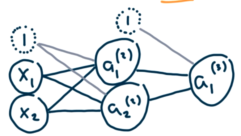
Thus, we can produce XOR by choosing \(\Theta\) values so that \(a_1^{(2)} \) evaluates the \(x_1\) OR \(x_2\) function and \(a_2^{(2)} \) evaluates the NOT(\(x_1\) AND \(x_2\)) and \(a_1^{(3)} \) evaluates the NOT(\(x_1\) AND \(x_2\)) \(a_1^{(2)} \) AND \(a_2^{(2)}. \)
The \(\Theta\) values for OR were -10,20,20. Thus,
The \(\Theta\) values for AND were -30,20,20. Thus,
In order to create the NOT of a function, we want to switch all the zeros to ones and all the ones to zeros. The simplest way to do that is to switch all the signs of the coefficients. So the \(\Theta\) values for NOT AND are 30,-20,-20. Thus,
This produces the three activation functions:
Let's check all the cases to show this works.
| \(x_1\) | \(x_2\) | \(a_1^{(2)} = g(-10+20x_1+20x_2)\) | \(a_2^{(2)}=g(30-20x_1-20x_2)\) | \(g(-30 +20a_1^{(2)}+20a_2^{(2)})\) |
| 0 | 0 | \(g(-10)=0\) | \(g(30)=1\) | \(g(-30+20)=0\) |
| 1 | 0 | \(g(-10+20)=1\) | \(g(30-20)=1\) | \(g(-30+20+20)=1\) |
| 0 | 1 | \(g(-10+20)=1\) | \(g(30-20)=1\) | \(g(-30+20+20)=1\) |
| 1 | 1 | \(g(-10+20+20)=1\) | \(g(30-20-20)=0 \) | \(g(-30+20)=0\) |
Subsection 9.2 Perceptrons
In the previous section, we discussed simple artificial neurons, but we didn't have a way to train the neurons using data. We could choose specific \(\Theta\) values to make the neuron behave like a logic gate, but of course, this isn't actually machine learning. In this section, we will discuss the idea of perceptrons and see how to train a model using data.
Recall, a neuron has an input layer, an output layer, and possibly any number of hidden layers, as in the image below.
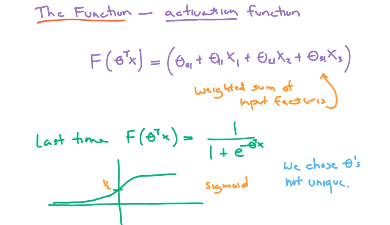
The activation function we used was a weighted sum of input features and the goal was to learn the weights, or choose the weights appropriately.
For a perceptron, also called a threshold logic unit (TLU), we will use a different activation. We will use a step function. Two options for a step function are the heaviside function and the sign function.
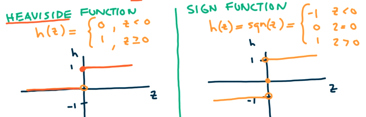
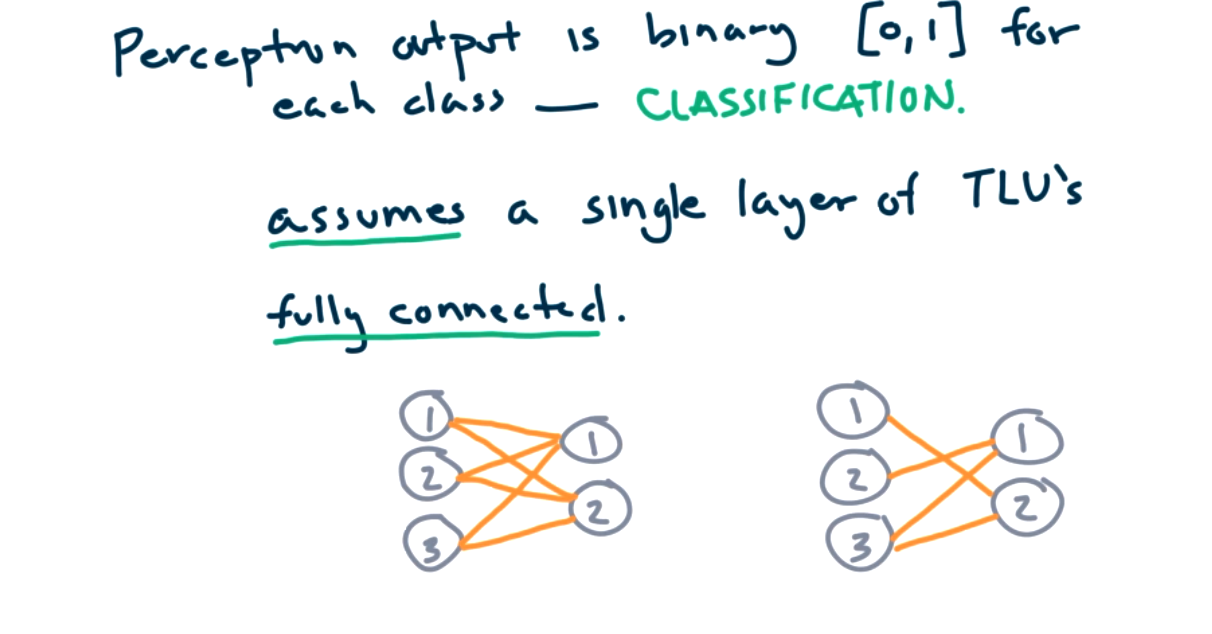
The changes we are making to move from an artificial neuron/logic gate model to a perceptron model include no hidden layers, changing the activation function from the sigmoid function to the heaviside step function, and the layers must be fully connected.
We will examine how to train a simple perceptron with two input features and two TLU's. Each TLU outputs either 0 or 1.
Example 9.7.
How do we use data to train a perceptron. The idea from neuroscience is "cells that fire together, wire together". The machine learning version is that the connection weight for \(\theta\) is larger for components that have a strong dependence on each other. We will train the perceptron by feeding one piece of data at a time, evaluating how well it predicts a classification, and updating the \(\theta\)s to improve the prediction. This requires labeled data so this is supervised learning. More specifically,
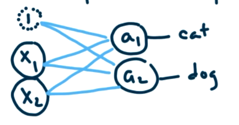
- Send in data \(x = \left[ \begin{matrix} x_1 \\ x_2 \end{matrix} \right]\)
- Perceptron makes prediction \(\hat{y} = \left[ \begin{matrix} a_1 \\ a_2 \end{matrix} \right]\)
- Compare the prediction to the correct classification \({y} = \left[ \begin{matrix} y_1 \\ y_2 \end{matrix} \right]\)
- Update each \(\theta_{ij} \) individually based on how closely the predictions matched the classifications. No change is needed if prediction is correct.
The update formula at the \(s+1\)th step for input unit \(i\) and output unit \(j\text{,}\) is given by
Note if the prediction is correct, \(y_j=a_j\) so the update term is 0 and \(\theta_{ij,s+1} = \theta_{ij,s}\text{.}\) If the prediction is incorrect, then the update term depends on the learning rate, \(\eta\text{.}\)
Let's see how to train our perceptron with one data point, where \(x = \left[ \begin{matrix} x_0 \\ x_1 \\ x_2 \end{matrix} \right] = \left[ \begin{matrix} 1 \\ 0.5 \\ 1 \end{matrix} \right]\text{.}\) Remember that \(x_0\) is the bias term which we always set to one. We will assume this data point corresponds to a cat so that \({y} = \left[ \begin{matrix} 1 \\ 0 \end{matrix} \right]\text{.}\) We need to initialize the \(\theta_{ij,0}\) to some value, so we will set them all equal to 1. There are two TLUs in our model, so we examine each one individually.
Remember that \(h\) is the heaviside step function so it outputs 1 as long as \(x \gt 0\text{.}\) Thus, \(a_1=y_1\) and our model predicts the correct answer.
In this case, \(a_2 \neq y_2\) and our model predicts the incorrect answer.
Let's apply our update function corresponding to step 1. We need to specify a learning rate. Generally we want this to be small, so we will pick \(\eta=0.1\text{.}\)
Since the prediction \(a_1\) is correct, \((y_j-a_j)=1-1=0\text{,}\) thus \(\theta_{01}=1, \theta_{11}=1, \theta_{21}=1\) remain unchanged. Let's consider \(\theta_{02,1}\text{.}\)
(x_0=bias term) \(=1+0.1(0-1)*1\) \(=1-0.1=.9\)
Question 9.8.
What should \(\theta_{12,1}\) and \(\theta_{22,1}\) be? Answer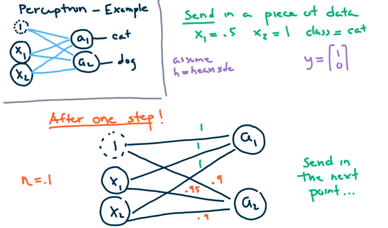
This update process is highly dependent on the size of \(x\) and \(\eta\text{.}\)
Question 9.9.
What should we do first? Answer
We can examine perceptrons via sklearn.
from sklearn.linear_model import Perceptron
We will still apply regularization in this model. Previously, the regularization penalty was in the cost function. We don't have that in this case, but we can still penalize large theta values during training.
Switch to Jupyter notebook!
Coming next time: Multilayer perceptrons! We want to create more complex models with multiple perceptrons. But the training is harder and we need backpropagation to update theta values. For a single perceptron, it was easy to solve for the thetas. With more layers, it will take a lot more work to trace back through all the hidden layers to update the theta values.
Subsection 9.3 Multi-Layer Perceptrons
How do we build neural networks from perceptrons? We need multilayer perceptrons, also known as deep neural networks. In this section we will provide an overview of training and architecture and an introduction to Keras.
How do we train a Neural Net with lots of hidden layers? Let's recall simple regression.
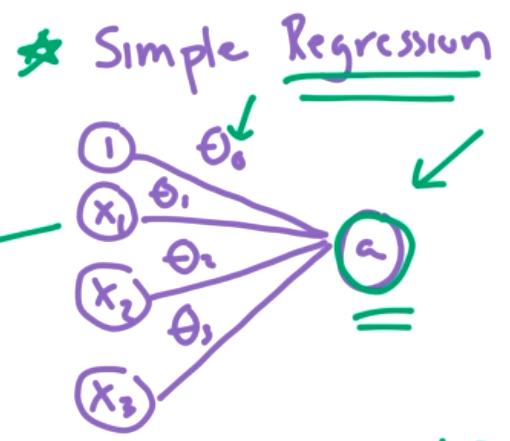
We could view this as a simple neural network. How did we do training here? We used gradient descent to minimize the cost function J. We updated the \(\Theta\) values with a learning rate and the slope/partial derivative of J with respect to the appropriate theta. That is,
new theta = old theta - (learning rate)(slope at J)
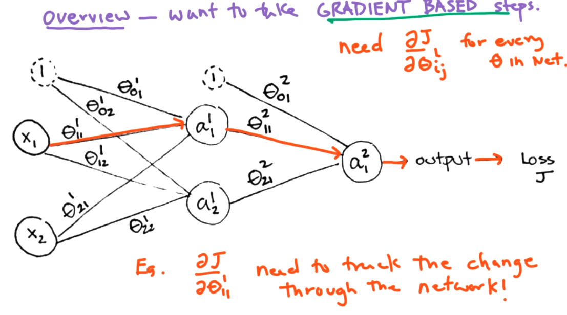
How does \(x_1\) affect the cost J? its just a single partial derivative, \(\frac{\partial{J}}{\partial{\theta_1}} .\)
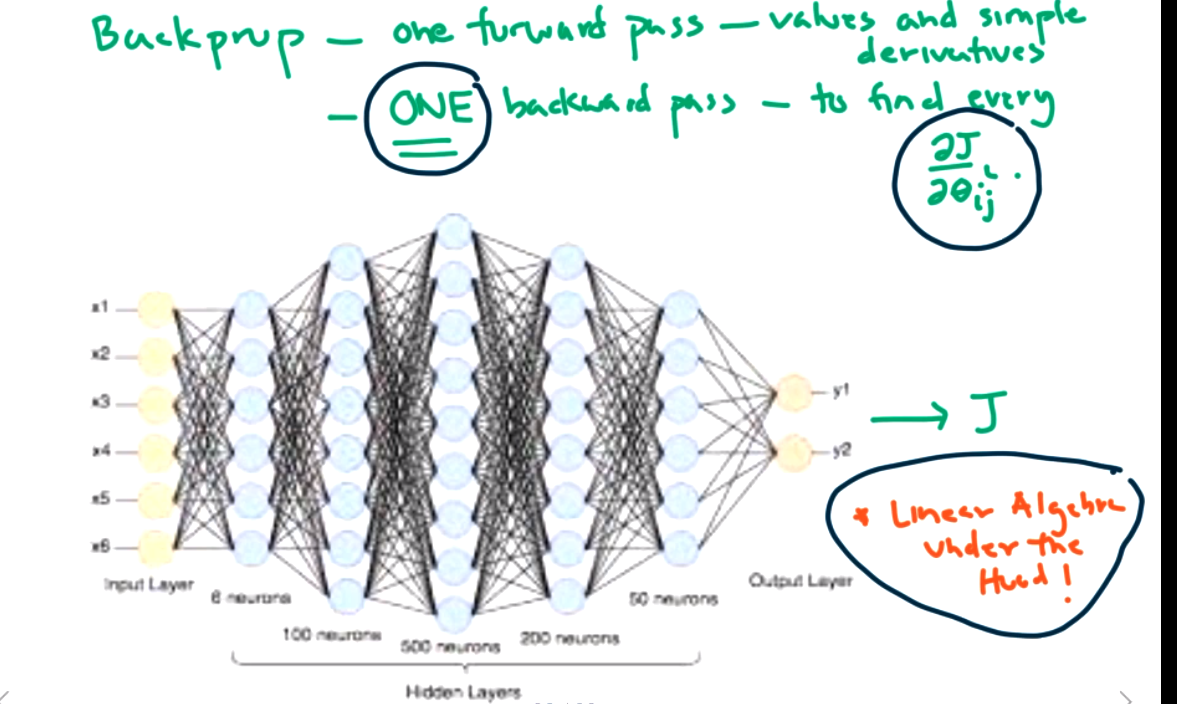
What does it mean in a deep neural network? We need a new cost function J, and we need to calculate many partial derivatives, \(\frac{\partial{J}}{\partial{\theta_{ij} ^n}} .\)
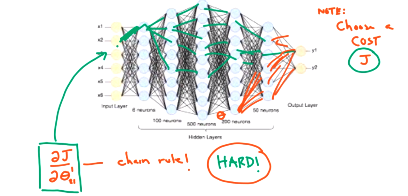
We will talk more about the details of backpropagation in the next section, but as an overview, there are two main steps to backpropagation.
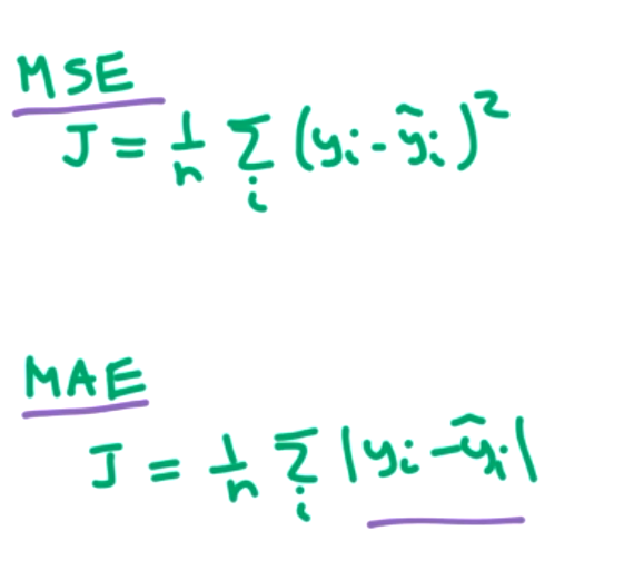
- Forward pass. Send a small batch of the data into the network. Keep track of each neuron's output. Calculate the cost using a measure of the network error, such as MSE, cross entropy loss, etc.
- Backward pass. Compute error due to each output. Calculate gradients of error going backward. Update each theta (similar to gradient descent technique).
- Repeat for each batch.
Each epoch corresponds to going through the entire data set, batch by batch, one time. Normally, we will go through through multiple epochs.
In the forward direction, we have to track all possible paths which is a lot. However, in the backward direction we can calculate each piece and store that, so its easier at the next step. We start closer to the cost function.
Things to keep in mind:
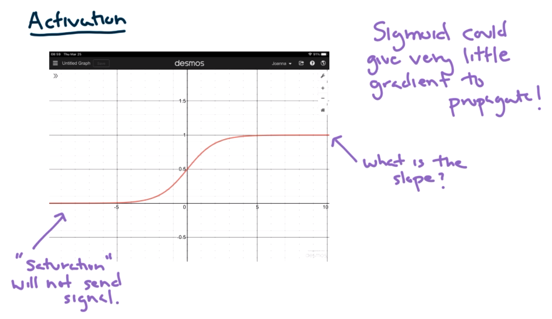
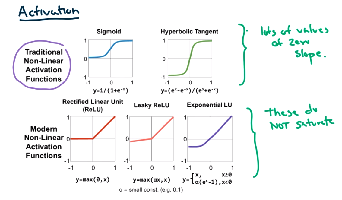
- We are taking derivatives, if we are using the heaviside step function as in the perceptrons, there is a point where the derivative is undefined, and the derivative is zero at most points. This is a problem. We need activation functions that have derivatives and have nonzero slope.
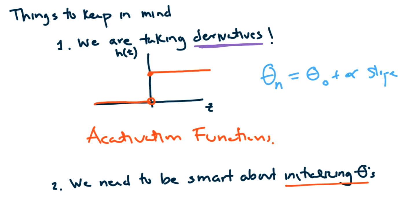
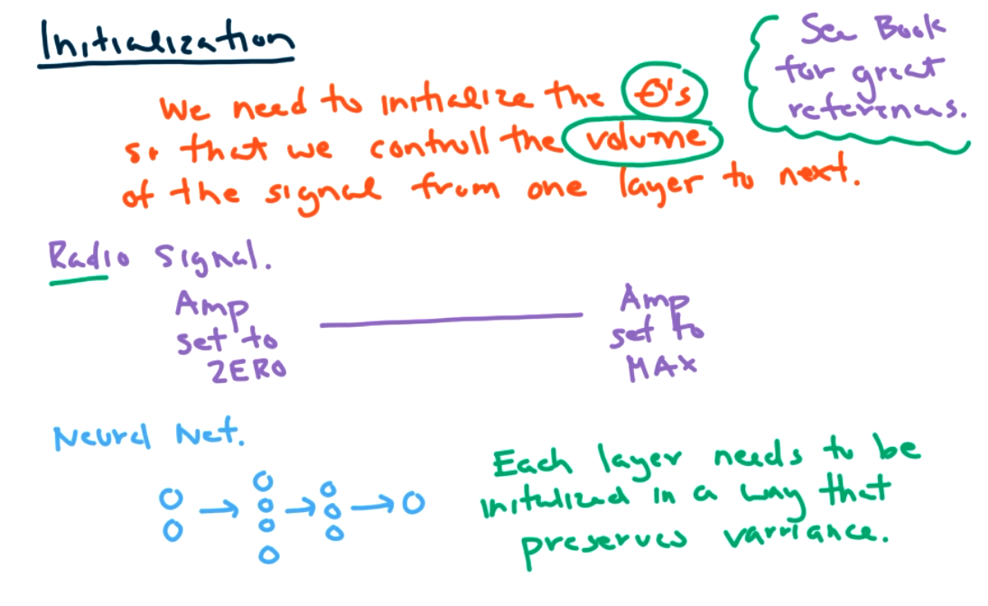
- We need to be smart about initializing thetas. We shouldn't initialize to zero, because it would be hard to learn. Normally we will initialize randomly between 0 and 1. Want to avoid certain symmetries. Dividing by zero issues can lead to convergence problems. There can also be issues based on the choice of initialization.
Some popular activation function are shown below.
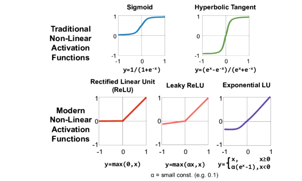
What is the output from an activation function? It will be any number between 0 and 1, so we will have to interpret for classification. It is important that the activation functions are non-linear. (See other class notes for an example of linear functions could be reduced to a single linear function.)
Can use deep neural networks for either regression or classification. In both cases we need to decide
- How many input neurons? (This should correspond to the numer of inputs.)
- How many hidden layers?
- How many neurons per hidden layer?
- How many output neurons? (If output is a single value, then only need one neuron here. But could have as many output neurons as things we want to predict. For example, an (x,y) location would have two outputs.)
- Output activation.
- Loss function.
For regression, there is usually no activation on the output. And typical loss functions are MSE or MAE. MAE is a little bit faster computationally for some cases.
For classification, most of the steps are the same. The main differences are in the cost function and activation function on OUTPUT layer. To get a classification we want the output to be 0 or 1. We can apply the logistic/sigmoid function at that step to classify.
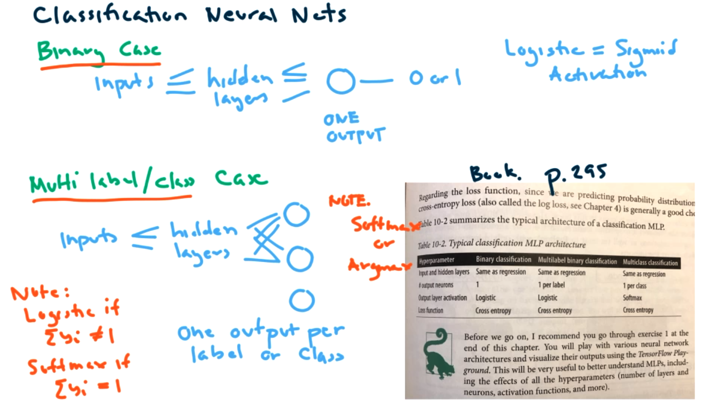
For the multiclass case, we will have one output per class. If we don't care about probability interpretation then logistic function is ok. If we do care about interpreting answers as a probability, then we should use the softmax function. Once we have all the outputs, we can apply softmax or argmax to see which class got the highest score, to predict a class.
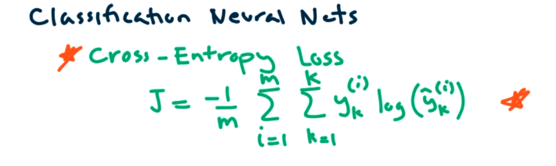
For the loss function, we want to use cross entropy loss. Remember we saw this before in logistic regression and if \(k=2\) then cross entropy loss reduces to the simpler logistic regression cost function (log-loss).
To implement Neural Networks, there are great packages!
Keras is great for building neural networks and the easiest place to start for experimentation. Keras builds a model one layer at a time. Easiest way is sequential model. Always assumes outputs from one layer are the input for the next layer. [More complex models in functional API]
Tensorflow and Pytorch are more advanced models. There are a lot more options to control here. (Keras is built on top of Tensorflow.)
Switch to Jupyter notebook for Keras example of simple neural net.
Subsection 9.4 Back Propagation
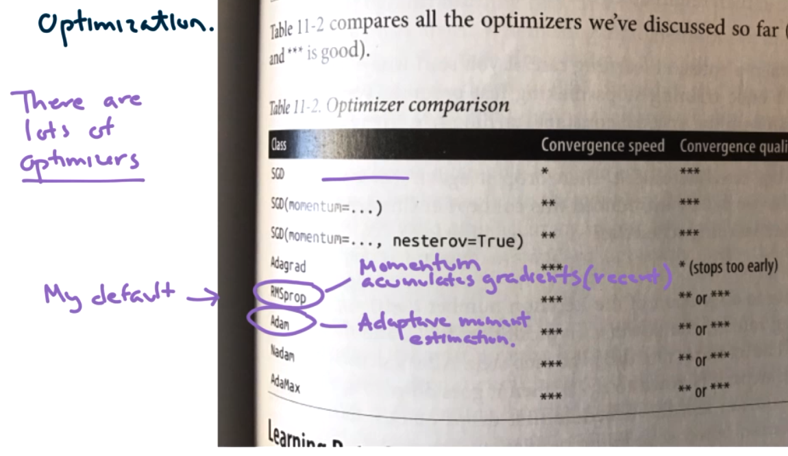
In this section we will introduce the concept of back propagation, its benefits and pitfalls, and a brief introduction to optimizers. The idea of back propagation is doing multivariable calculus on a graph. It makes training much, much faster on the scale of reducing the time from 200,000 years to one week. Its an important reason why neural networks have become so powerful. A full discussion of optimizers would involve lots of linear algebra and multivariable calculus. We aren't going to go through all of those details, but encourage you to research those details! (See references in your text.)
Remember that the goal in a neural network is to find \(\Theta\) values that minimize a loss function \(J\text{.}\)
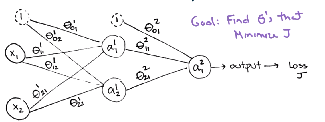
As part of training, we want to update all of the \(\Theta\) values based on partial derivatives, \(\frac{\partial J}{\partial \theta_{ij}^L}\text{.}\)
We will need partial derivatives from Calculus, so we will include a quick reminder of what partial derivatives are. Suppose we have a function of two variables, \(f(x,y)=2x+3y+xy\text{.}\) Since there are two variables, we can take the derivative with respect to either \(x\) or \(y\text{.}\) The idea is to treat the other variable as a constant.
Example 9.10.
Compute \(\frac{\partial f}{\partial x}\) for \(f(x,y)=2x+3y+xy\text{.}\) We treat \(y\) as a constant in this case. So \(\frac{\partial f}{\partial x}=2+0+y.\)
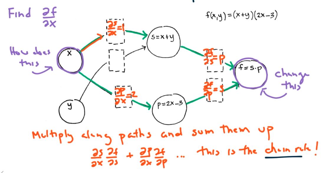
The next idea we need is the chain rule for partial derivatives. We can think of the chain rule as a mobster who needs to shake down every term to get the needed information. In this case, we consider a function \(f(g,h)\) where \(g,h\) are both function of two variables \(x\) and \(y\text{.}\) That is, \(g(x,y)\) and \(h(x,y)\text{.}\) The chain rule for partial derivatives is
Both \(g(x,y)\) and \(h(x,y)\) have to give information about \(x\text{.}\)
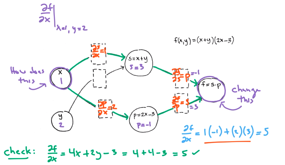
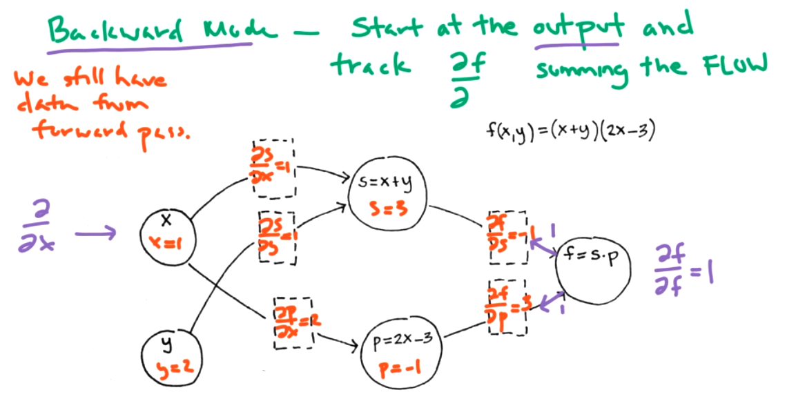
Example 9.11.
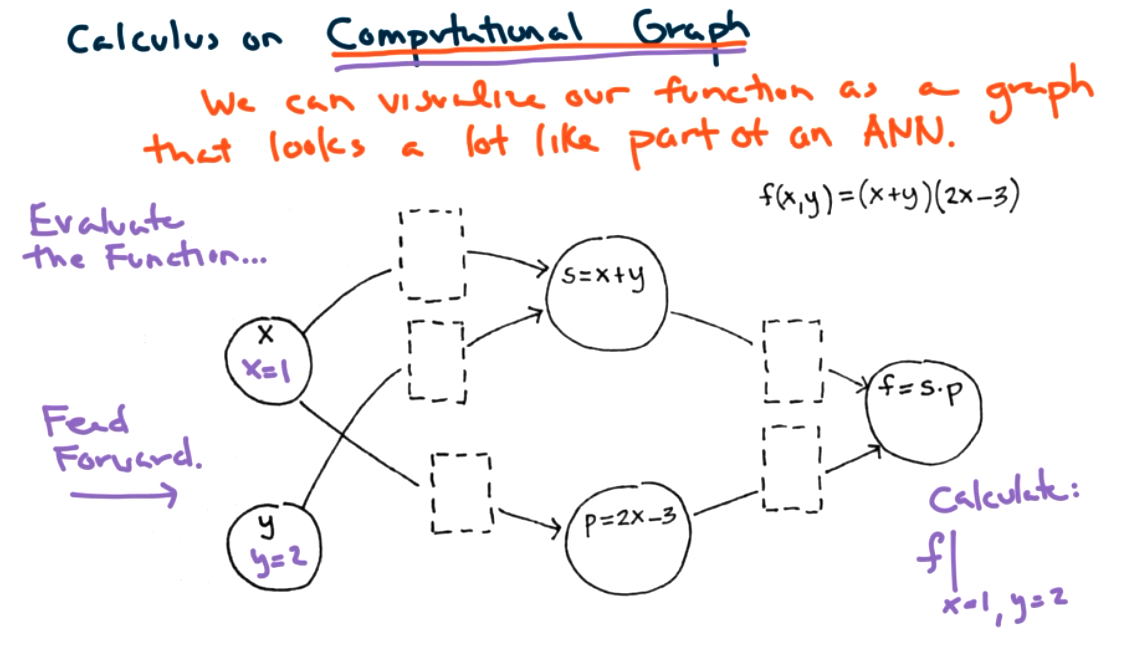
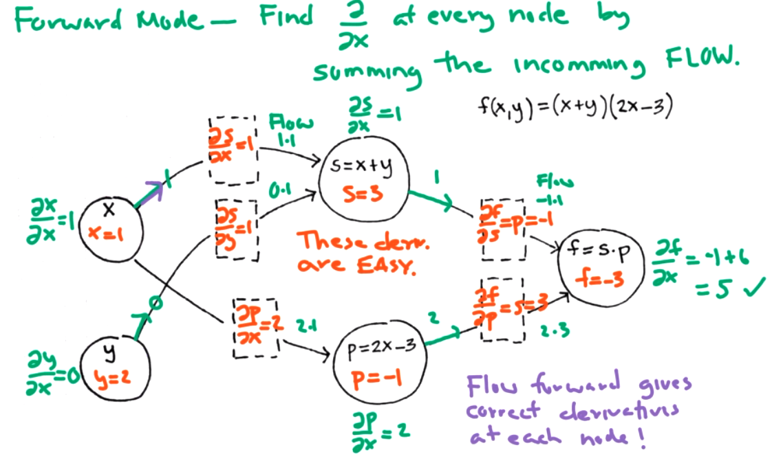
Suppose \(f(x,y) = s(x,y) p(x)\) where \(s(x,y)=x+y\) and \(p(x)=2x-3\text{.}\) There are two ways we can calculate derivates, we can use the chain rule or we can use algebraic simplification. For the chain rule
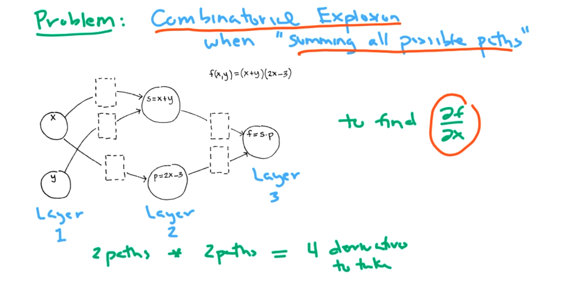
We can visual the functions and derivatives as a graph to connect this idea to neural networks. The chain rule is easier for computer. Algebraic simplificaiton requires symbolic algebra. The functions correspond to nodes.
- forward-mode differentiations
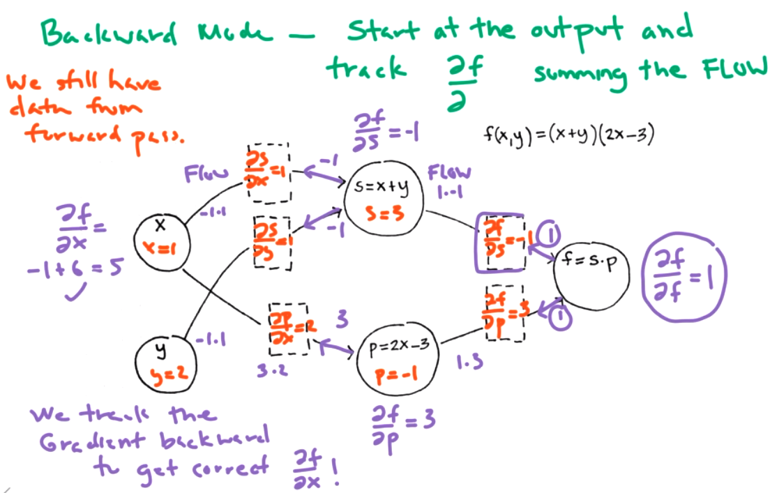
- backward-mode differentiation (Also called backprop or reverse node.)
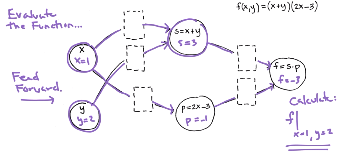
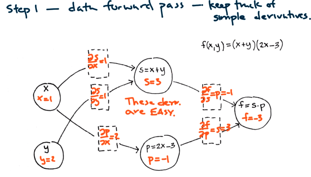
Both modes can help us find \(\frac{\partial f}{\partial x}\) at a point \((x,y)=(1,2)\text{.}\) Step 1: data forward pass -- keep track of simple derivatives store information about simple derivatives.

Question 9.12.
What is \(\frac{\partial f}{\partial y}\) for the same graph?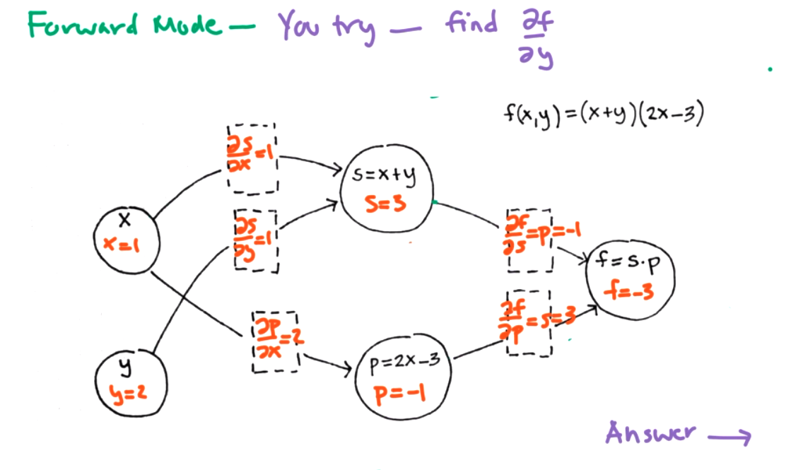
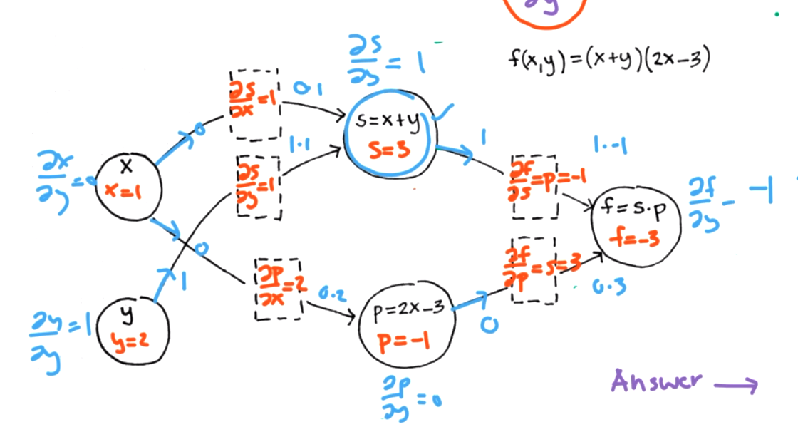
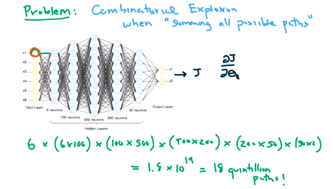
This is better than redoing the derivative each time, but its still a lot of work in a large network.
- Vanishing Gradients.
- Exploding Gradients
- Unstable Gradients
In the case of vanishing gradients, one of the activations doesn't send a very strong signal. That is, small partial derivatives at some layer. Remember that the idea of gradients is that we are hiking down a hill into a valley proportional to the steepness of a hill. If we hit a flat point, then there won't be any update to that theta value. The algorithm might not converge, or will take a long time.
For the case of exploding gradients, this can easily diverge since we are likely to take way too big of a step. Or it could take longer to converge.
For the case of unstable gradients, different layers are learning at different rates. It is difficult to pick a learning rate that works for all of these layers.
We need our signal to flow forward to give us a prediction, but backward to get an update. Need signal to flow in both directions. Makes it hard to choose a good initialization and the activation function has a huge impact on neural net. see book for references. Here's the idea:
Subsection 9.5 Keras and Tensorflow
Review of sequential model functional model callback -- keep track of runs and keep best one visualization tool called tensorboard Regression Neural Net and Keras Tools copy from notebook?? Idea of sequential model is that one layer flows to the next and all inputs are used. bias term 8+1 * 30 + 31*1 parameters model = keras.models.Sequential([ each layer]) model.compile() SGD ok because model is simple. history=model.fit() what should we see in loss? decrease but could increase a little stochastic gradient descent might move a little randomly model.evaluate(testing data) Functional API think about layers as functions, so we specify input not just assume all entries from last layer. We can think about deep and wide, some features could go deep (many hidden layers) or wide (not through all layers) keras.backend.clear_session() input_ = keras.layers.Input(shape=X_train_s.shape) hidden1=keras.layers.Dense(30, activ)(input_) hidden2=keras.layers.Dense(hidden1) concat=keras.layers.concatenate([input_,hidden2]) output=keras.layers.Dense(1)(concat) model= keras.models.Model(inputs=[input_],outputs=[output]) When wide and when deep? based on data but mostly experimentation Could help if we had really different types of data that we wanted to use for a single answer. Maybe voice data and image data. Really helpful tools saving and restoring a model -- keep good notes about what you are trying while experimenting -- it can take a long time to train and don't want to redo that -- model.save("name.h5") keras.models.load_model("name.h5") save model in the .fit command. callback build model, compile name_cb=keras.callbacks.ModelCheckpoint("best",save_best_only=True) model.fit( ..., callbacks=[name_cb]) There's a lot more to play with here! Explore the documentation!! Tensorboard Pretty cool!Subsection 9.6 Hyperparameter Tuning
Today we will learn about a few tools for fine tuning our neural network models. If you are training neural networks professionally then you should absolutely read chapter 11 along with all of the papers referenced in chapter 11.
Hyperparameter Tuning
- GridSearchCV or RandomizedSearchCV are usefull if you wrap your model in sklearn
What are some important parameters:
- Number of Hidden Layers
- Number of Neurons Per Layer
- Learning Rate
- Optimizer Used
- Batch Size
- Activiation Functions
- Numnber of Epochs
Regularization
- If you are training a very complicated neural network you almost always want to add in some regularization!
Types of regularization
- Simple L1 and L2 - same as before applied during training
- Dropout - drop neurons during training with some probability - all neurons used during prediction
- Monte Carlo Dropout - boosts preformance of a trained dropout model - applied after training during prediction
- Max-Norm - a special way of rescaling after each training step
See Jupyter Notebook.
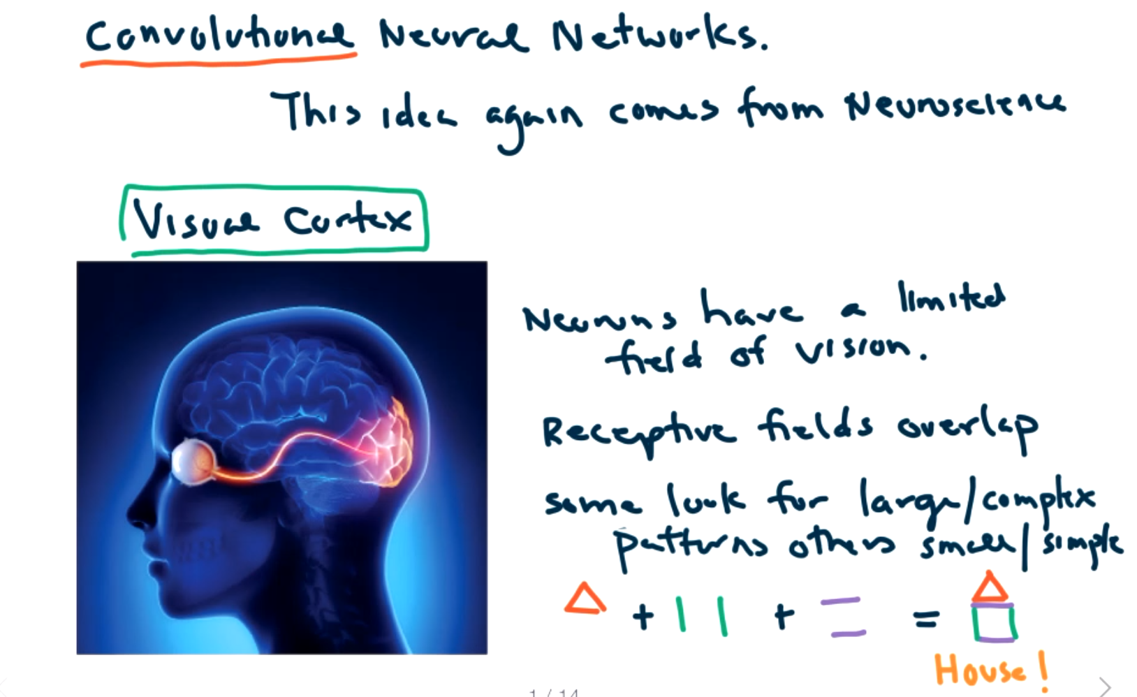
Subsection 9.7 Convolutional Neural Network
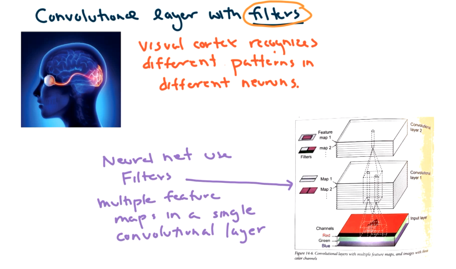
The idea again comes from neuroscience and examining the visual cortex.
- Each individual neuron has a limited field of vision.
- Receptive fields overlap.
- Some look for larger/complex patterns and others will look for small/simple details.
Can we do this with an artificial neural network? In fact, we can! Le Cun presented this idea for what are called convolutional neural networks (or CNN) in 1988. But needed more powerful computers and more labeled data for it to take off and become useful.
The convolutional layer represents the visual cortex. We connect this to a deep fully connected neural network to do the decision making.
But wait! Haven't we already done image classification with deep NN? MNIST has very small images that are extremely simple. So a plain NN worked ok. But it won't work as well for larger, more complex images.
If we wanted to send a 100 by 100 image through a traditional neural network, we must first flatten it to an 10000 array. This can be connected to any number of neurons in the first layer, say 1000. This is a huge parameter set.
Its worse than that though! We are losing the spatial connection between pixels. Its really hard to identify images from isolated pixels. We really need to know how the pixels are connected.
Convolution is a mathematical operation. For example, the Laplace transform features the integral of pointwise multiplication.
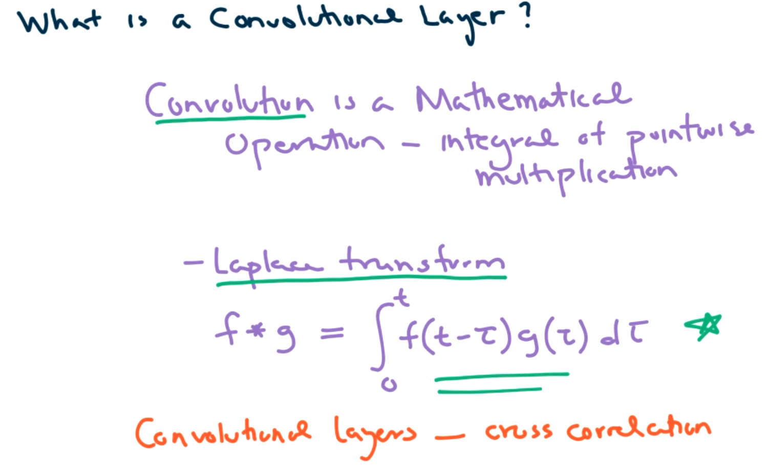
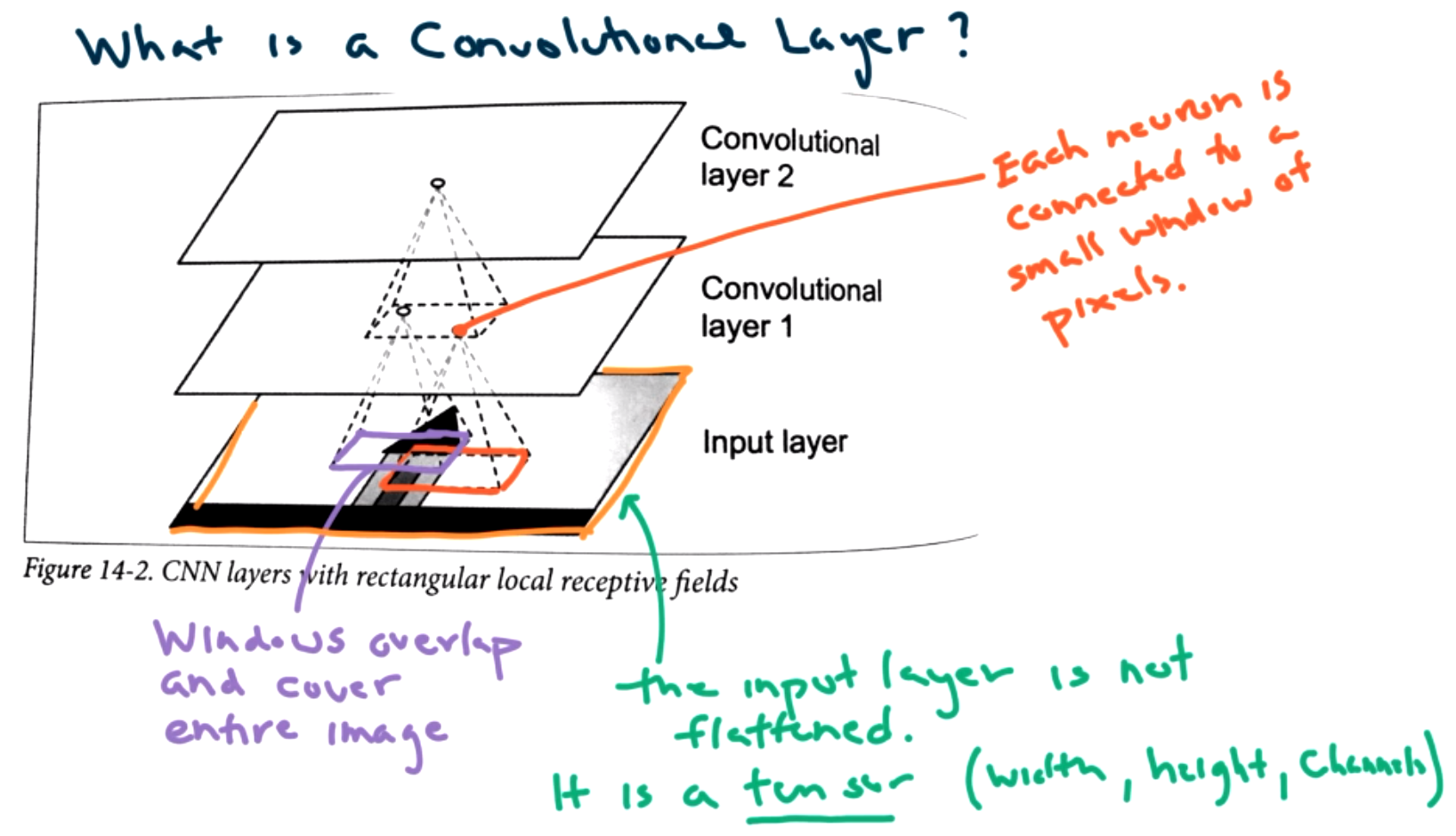
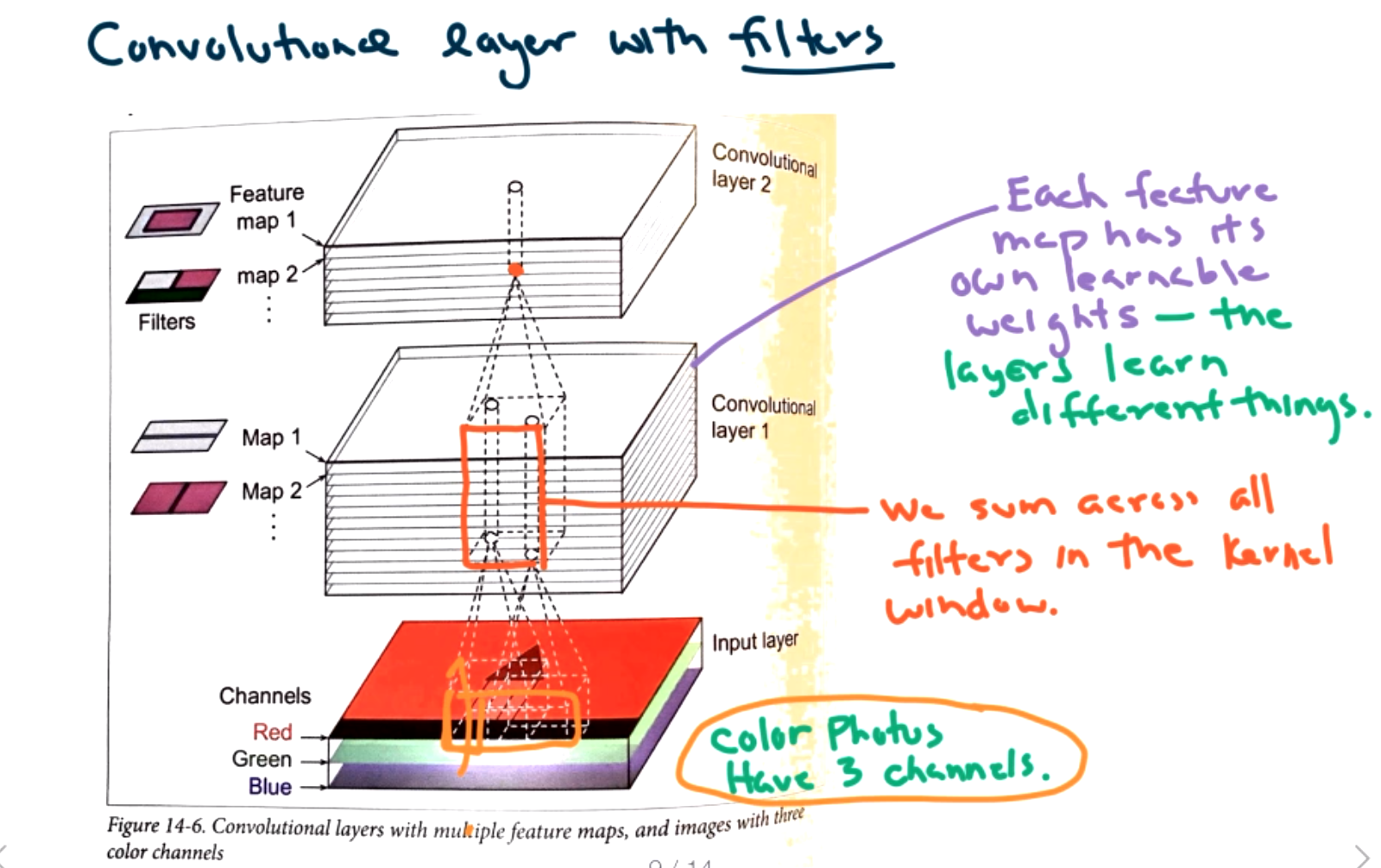
What is a convolutional layer? Each convolutional layer maps a subset of the image to a single neuron in the next layer. Each neuron is connected to a small window of pixels. The windows overlap and cover the entire image. Convolutional layers may or may not reduce the size in the layers depending on how the windows overlap. The input layer is not flattened. It is a tensor. (contains width, height, certain number of channels) The number of channels depends on the color (1 channel for gray scale, 3 channels for RGB, all layered on top of each other.)
More specifically we examine a convolutional layer in
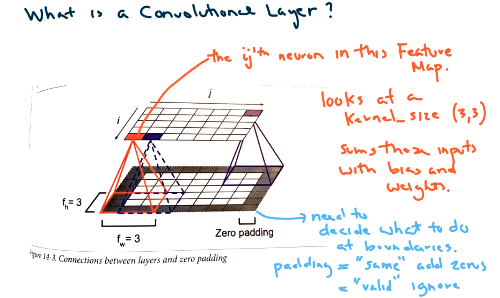
One issue that must be decided is what to do at the boundaries of the image. We could fill with zeros (padding="same") or we could ignore the boundary points (padding="valid").
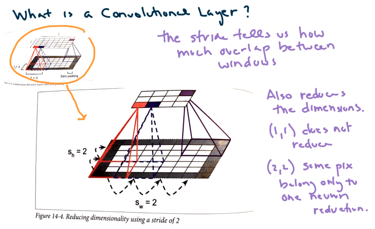
The next question is how big of a step should we take.
The next idea is filters.
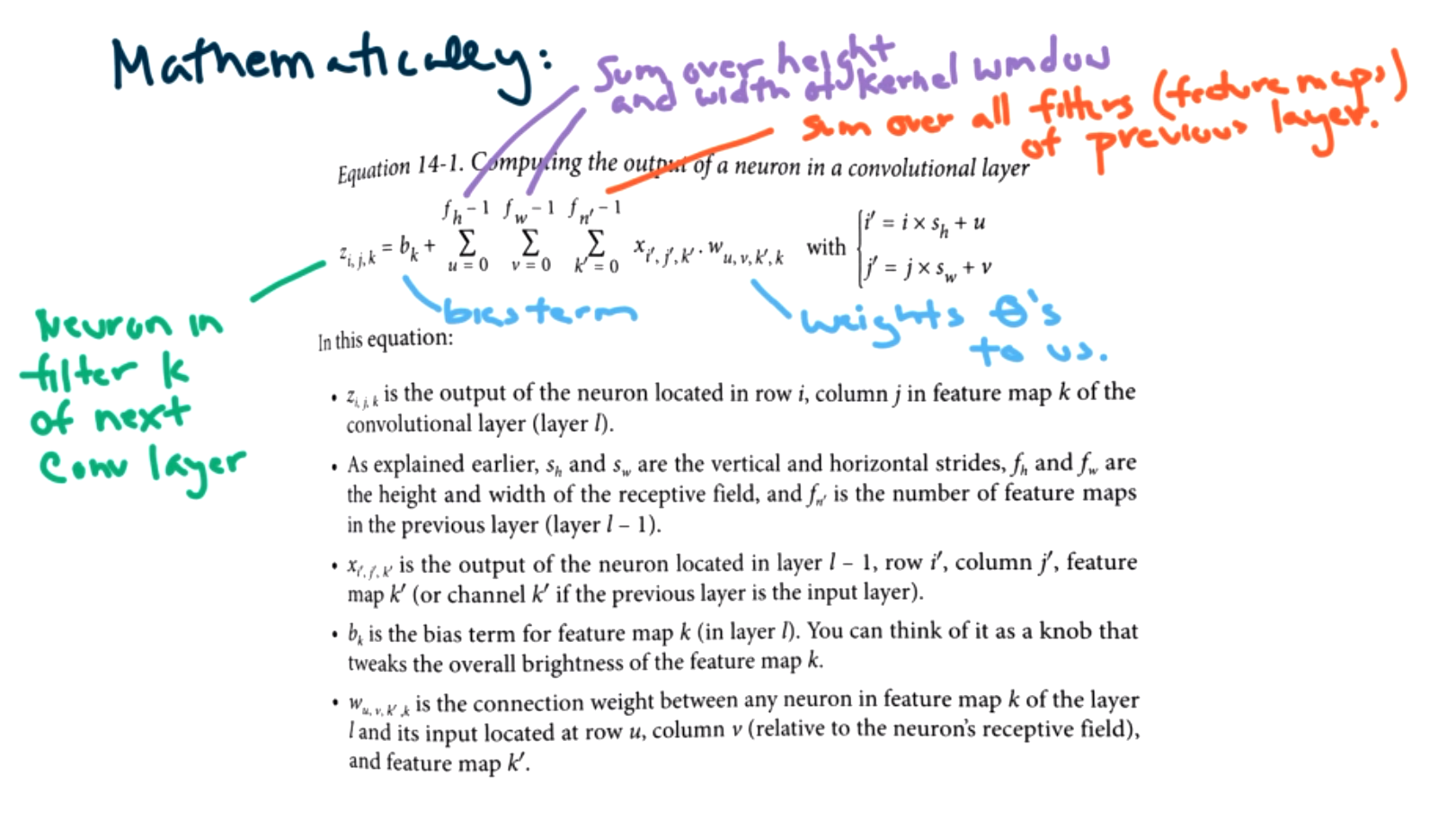
The Math! If we want to calculate what is happening in neuron \(i,j \) we must sum over height and width of kernel window and sum over all the filters.
Convolutional neural nets work really well, but they require a huge amount of memory for large images! This is especially a problem for back propagation since we had to keep so many terms in memory. It is easy to run into memory errors. There are some fixes for this:
- small batch size
- increase stride to reduce dimension
- 16 bit vs 32 bit floats (save less decimal places)
- distribute data across multiple machines/processors
- pooling layers
What are pooling layers? The idea is to pool data to reduce dimensionality.
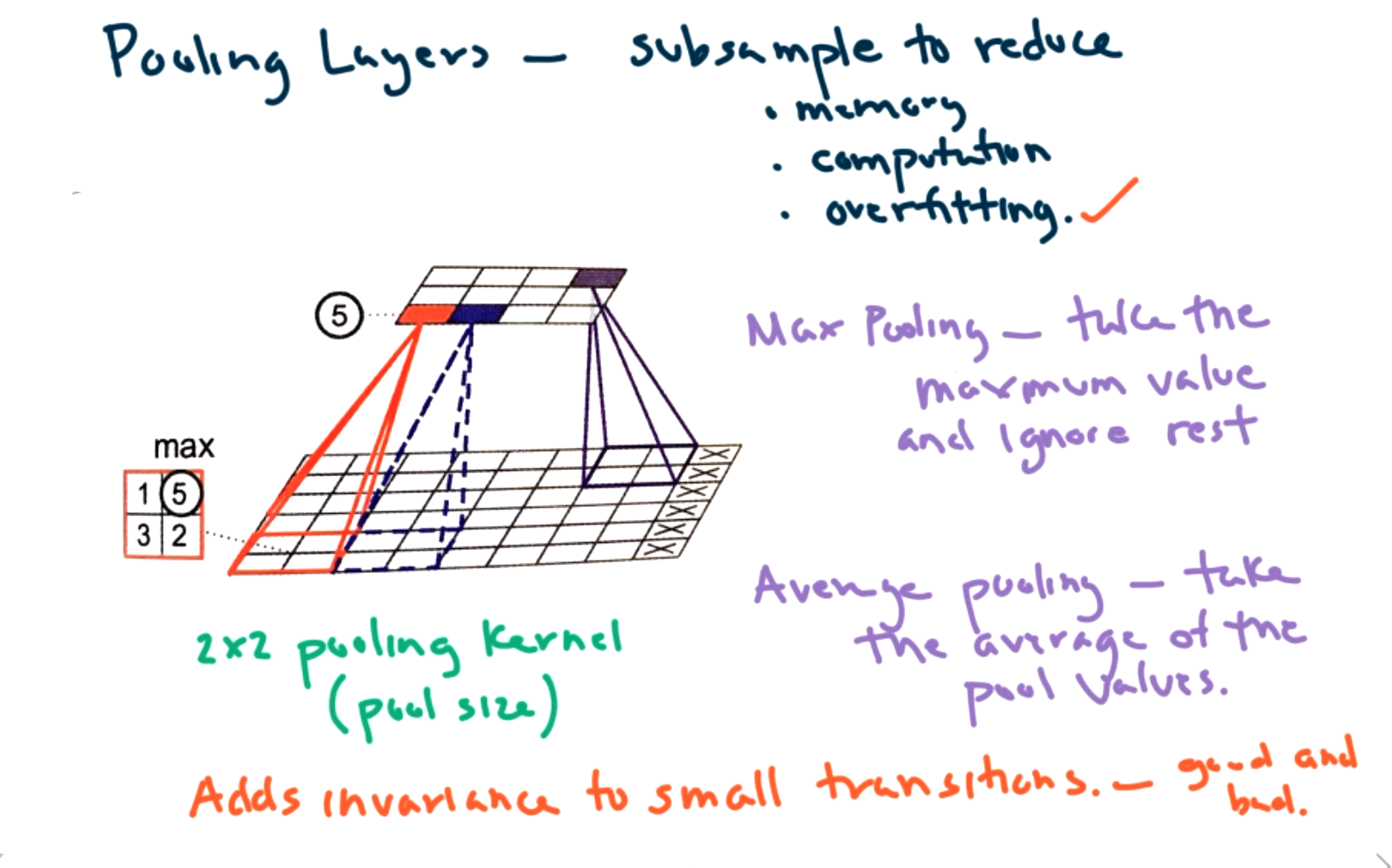
- memory
- computation
- overfitting
There are two main ways to apply pooling. We can use either max pooling or average pooling. In max pooling, take the maximum value and ignore the rest. That is, examine each window and find the max. For average pooling, take the average of the values in the window.
One consequence of pooling is to add invariance to small transitions. This can be both good and bad. For example, if you want to classify a dog in the snow, you might want to ignore small bits of snow on the dog. Of course, if you want to identify that it is snowing, then you won't want to ignore that information.
We do still want to apply regularization in CNN. We can use kernel regulizers as before specifying either l1 or l2 norms. Dropout can also be applied, but it must be done differently because of the spatial data. We don't want to drop out parts of the image, instead we will probabilistically drop out entire feature maps.
An example of a full CNN is pictured below.
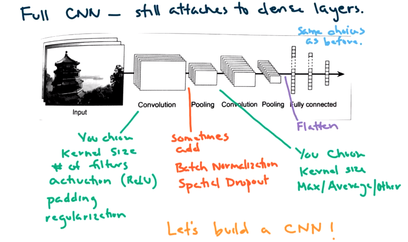
There are a number of decisions to make:
- kernel size
- # of filters
- activation
- padding
- regularization
Sometimes we add normalization and regularization between convolutional and pooling layers.
Sometimes batch normalization is used to help avoid exploding gradients. We would just apply this after the first convolutional layer.
For pooling layer you must specify the kernel size and the type of pooling (max or average).
You can have as many convolutional and pooling layers as you want. Then flatten and send through a traditional deep NN as before.
Time for example in Jupyter notebook. Follows blog -- check it out.